Orbital optimization

The radial function of basis orbitals can be variationally optimized using the orbital optimization method [30]. As an illustration of the orbital optimization, let us explain it using a methane molecule of which input file is 'Methane_OO.dat'. In the orbital optimization method the optimized orbitals are expressed by the linear combination of primitive orbitals, and obtained by variationally optimizing the contraction coefficients. The number of the primitive and optimized orbitals in the optimization are specified by

    <Definition.of.Atomic.Species
      H   H5.0-s4>1            H_CA13
      C   C5.0-s4>1p4>1        C_CA13
    Definition.of.Atomic.Species>

For 'H' one optimized radial function for the s-orbital is obtained from the linear combination of four primitive radial functions. Similarly, one optimized radial function for the s-(p-)orbital is obtained from the linear combination of four primitive radial functions for 'C'. In addition, the following keywords are set in the input file as follows:

    orbitalOpt.Method          species     # Off|Species|Atoms
    orbitalOpt.Opt.Method        EF        # DIIS|EF
    orbitalOpt.SD.step        0.001        # default=0.001
    orbitalOpt.HistoryPulay     30         # default=15
    orbitalOpt.StartPulay       10         # default=1
    orbitalOpt.scf.maxIter      60         # default=40
    orbitalOpt.Opt.maxIter     140         # default=100
    orbitalOpt.per.MDIter       20         # default=1000000
    orbitalOpt.criterion      1.0e-4       # default=1.0e-4 

    CntOrb.fileout               on        # on|off, default=off
    Num.CntOrb.Atoms             2         # default=1
    <Atoms.Cont.Orbitals
     1
     2
    Atoms.Cont.Orbitals>

Then, we execute OpenMX as:

    % ./openmx Methane_OO.dat
  

When the execution is completed normally, you can find the history of orbital optimization in the file 'met_oo.out' as:

***********************************************************
***********************************************************
         History of orbital optimization   MD= 1
*********     Gradient Norm ((Hartree/borh)^2)     ********
              Required criterion=  0.000100000000
***********************************************************

   iter=   1  Gradient Norm=  0.057098961101  Uele= -3.217161102876
   iter=   2  Gradient Norm=  0.044668461503  Uele= -3.220120116009
   iter=   3  Gradient Norm=  0.034308306321  Uele= -3.223123238394
   iter=   4  Gradient Norm=  0.025847573248  Uele= -3.226177980300
   iter=   5  Gradient Norm=  0.019106400842  Uele= -3.229294858054
   iter=   6  Gradient Norm=  0.013893824906  Uele= -3.232489198284
   iter=   7  Gradient Norm=  0.010499500005  Uele= -3.235304178159
   iter=   8  Gradient Norm=  0.008362635043  Uele= -3.237652870812
   iter=   9  Gradient Norm=  0.006959703539  Uele= -3.239618540761
   iter=  10  Gradient Norm=  0.005994816379  Uele= -3.241268535418
   iter=  11  Gradient Norm=  0.005298095979  Uele= -3.242657118263
   iter=  12  Gradient Norm=  0.003059655878  Uele= -3.250892948269
   iter=  13  Gradient Norm=  0.001390201488  Uele= -3.255123241210
   iter=  14  Gradient Norm=  0.000780925380  Uele= -3.255179362845
   iter=  15  Gradient Norm=  0.000726631072  Uele= -3.255263012792
   iter=  16  Gradient Norm=  0.000390930576  Uele= -3.250873416989
   iter=  17  Gradient Norm=  0.000280785975  Uele= -3.250333677139
   iter=  18  Gradient Norm=  0.000200668585  Uele= -3.252345643243
   iter=  19  Gradient Norm=  0.000240367596  Uele= -3.254238199726
   iter=  20  Gradient Norm=  0.000081974594  Uele= -3.258146794679

In most cases, 20-50 iterative steps are enough to achieve a sufficient convergence. The comparison between the primitive basis orbitals and the optimized orbitals in the total energy is given by

    Primitive basis orbitals
       Utot  =      -7.992569945749 (Hartree) 

    Optimized orbitals by the orbital optimization 
       Utot  =      -8.133746986502 (Hartree)

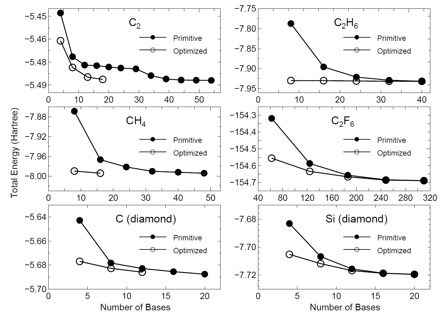
We see that the small but accurate basis set orbitals can be generated by the orbital optimization. In Fig. 16 we show the convergence properties of total energies for molecules and bulks as a function of the number of unoptimized and optimized orbitals, implying that a remarkable convergent results are obtained using the optimized orbitals for all the systems. In this illustration of a methane molecule, the optimized radial orbitals are output to files 'C_1.pao' and 'H_2.pao'. These output files 'C_1.pao' and 'H_2.pao' could be an input data for pseudo-atomic orbitals as is. This means that it is possible to perform a pre-optimization of basis orbitals for systems you are interested in. The pre-optimization could be performed for smaller but chemically similar systems.

The following two options are available for the keyword 'orbitalOpt.Method': 'atoms' in which basis obitals on each atom are fully optimized, 'species' in which basis obitals on each species are optimized.

• atoms

  The radial functions of basis orbitals are optimized with a constraint that the radial wave function $R$ is independent of the magnetic quantum number, which guarantees the rotational invariance of the total energy. However, the optimized orbital on all the atoms can be different from eath other.

• species

  Basis orbitals in atoms with the same species name, that you define in 'Definition.of.Atomic.Species', are optimized as the same orbitals. If you want to assign the same orbitals to atoms with almost the same chemical environment, and optimize these orbitals, this scheme could be quite convenient. As well as 'atoms', the optimized radial functions are independent of the magnetic quantum number, which guarantees the rotational invariance of the total energy.

Although the same information is available in the section 'Input file', for convenience the details of the other keywords are listed below:
orbitalOpt.scf.maxIter
The maximum number of SCF iterations in the orbital optimization is specified by the keyword 'orbitalOpt.scf.maxIter'.

orbitalOpt.Opt.maxIter
The maximum number of iterations for the orbital optimization is specified by the keyword 'orbitalOpt.Opt.maxIter'. The iteration loop for the orbital optimization is terminated at the number specified by 'orbitalOpt.Opt.maxIter' even when a convergence criterion is not satisfied.

orbitalOpt.Opt.Method
Two schemes for the optimization of orbitals are available: 'EF' which is an eigenvector following method, 'DIIS' which is the direct inversion method in iterative subspace. The algorithms are basically same as for the geometry optimization. Either 'EF' or 'DIIS' is chosen by the keyword, 'orbitalOpt.Opt.Method'.

orbitalOpt.StartPulay
The quasi Newton method, 'EF' and 'DIIS' starts from the optimization step specified by the keyword 'orbitalOpt.StartPulay'.

orbitalOpt.HistoryPulay
The keyword 'orbitalOpt.HistoryPulay' specifies the number of previous steps to estimate the next input contraction coefficients used in the quasi Newton method, 'EF' and 'DIIS'.

orbitalOpt.SD.step
Steps before moving the quasi Newton method, 'EF' and 'DIIS' is performed by the steepest decent method. The prefactor used in the steepest decent method is specified by the keyword 'orbitalOpt.SD.step'. In most cases, orbitalOpt.SD.step of 0.001 can be a good prefactor.

orbitalOpt.criterion
The keyword 'orbitalOpt.criterion' specifies a convergence criterion ((Hartree/borh)$^2$) for the orbital optimization. The iterations loop is finished when a condition, Norm of derivatives$<$orbitalOpt.criterion, is satisfied.

CntOrb.fileout
If you want to output the optimized radial orbitals to files, then the keyword 'CntOrb.fileout' must be ON.

Num.CntOrb.Atoms
The keyword 'Num.CntOrb.Atoms' gives the number of atoms whose optimized radial orbitals are output to files.

Atoms.Cont.Orbitals
The keyword 'Atoms.Cont.Orbitals' specifies the atom number, which was given by the first column in the specification of the keyword 'Atoms.SpeciesAndCoordinates' for the output of optimized orbitals as follows:

    <Atoms.Cont.Orbitals
     1
     2
    Atoms.Cont.Orbitals>

The beginning of the description must be '$<$Atoms.Cont.Orbitals', and the last of the description must be 'Atoms.Cont.Orbitals$>$'. The number of lines should be consistent with the number specified in the keyword 'Atoms.Cont.Orbitals'. For example, the name of files are 'C_1.pao' and 'H_2.pao', where the symbol corresponds to that given by the first column in the specification of the keyword 'Definition.of.Atomic.Species' and the number after the symbol means that of the first column in the specification of the keyword 'Atoms.SpeciesAndCoordinates'. These output files 'C_1.pao' and 'H_2.pao', can be an input data for pseudo-atomic orbitals as is.

Figure 16: The total energy for a carbon dimer C$_2$, a methane molecule CH$_4$, carbon and silicon in the diamond structure, a ethane molecule C$_2$H$_6$, and a hexafluoro ethane molecule C$_2$F$_6$ as a function of the number of primitive and optimized orbitals. The total energy and the number of orbitals are defined as those per atom for C$_2$, carbon and silicon in the diamond, and as those per molecule for CH$_4$, C$_2$H$_6$, and C$_2$F$_6$.