Band dispersion

The band dispersion is calculated by the following two steps:

(1) SCF calculation

Let us illustrate the calculation of band dispersion using the carbon diamond. In a file Cdia.dat in the directory 'work', the atomic coordinates, cell vectors, and scf.Kgrid are given by

    Atoms.Number         2
    Atoms.SpeciesAndCoordinates.Unit   Ang # Ang|AU
    <Atoms.SpeciesAndCoordinates           
     1   C  0.000  0.000  0.000   2.0 2.0
     2   C  0.890  0.890  0.890   2.0 2.0
    Atoms.SpeciesAndCoordinates>
    Atoms.UnitVectors.Unit             Ang # Ang|AU
    <Atoms.UnitVectors                     
      1.7800  1.7800  0.0000
      1.7800  0.0000  1.7800
      0.0000  1.7800  1.7800
    Atoms.UnitVectors>

    scf.Kgrid                  7 7 7       # means n1 x n2 x n3

The unit cell for the band dispersion and k-paths are given by

    Band.dispersion             on        # on|off, default=off
    <Band.KPath.UnitCell
     3.56  0.00  0.00
     0.00  3.56  0.00
     0.00  0.00  3.56
    Band.KPath.UnitCell>
    Band.Nkpath                  5
    <Band.kpath                
      15  0.0 0.0 0.0   1.0 0.0 0.0   g X
      15  1.0 0.0 0.0   1.0 0.5 0.0   X W
      15  1.0 0.5 0.0   0.5 0.5 0.5   W L
      15  0.5 0.5 0.5   0.0 0.0 0.0   L g
      15  0.0 0.0 0.0   1.0 1.0 0.0   g X 
    Band.kpath>

Then, we execute OpenMX by:

    % ./openmx Cdia.dat
  

When the execution is completed normally, then you can find a file 'cdia.Band' in the directory 'work'. When 'Band.KPath.UnitCell' does not exist, the unit cell specified by the 'Atoms.UnitVectors' will be used. Then, it is noted that '0.5 0.0 0.0' corresponds to the 'X'-point

(2) Converting of the data to a gnuplot form

Figure: Band dispersion of carbon diamond. The input file is Cdia.dat in the directory 'work'.

There is a file 'bandgnu13.c' in the directory 'source'. Compile the file as follows:

    % gcc bandgnu13.c -lm -o bandgnu13
  

When the compile is completed normally, then you can find an executable file, bandgnu13, in the directory 'source'. Please copy the executable file to the directory 'work'. Using the executable file 'bandgnu13' a file 'cdia.Band' is converted in a gnuplot format as

    % ./bandgnu13 cdia.Band	
  

Then, three or two files 'cdia.GNUBAND' and 'cdia.BANDDAT1' ('cdia.BANDDAT2') are generated. The file 'cdia.GNUBAND' is a script for gnuplot, and read data files 'cdia.BANDDAT1' and 'cdia.BANDDAT2' for up- and down-spin, respectively. If spin-polarized calculations using 'LSDA-CA' or 'LSDA-PW' is employed in the SCF calculation, '*.BANDDAT2' for down-spin is generated in addition to '*.BANDDAT1'. The file 'cdia.GNUBAND' is plotted using gnuplot as follows:

    % gnuplot cdia.GNUBAND
  

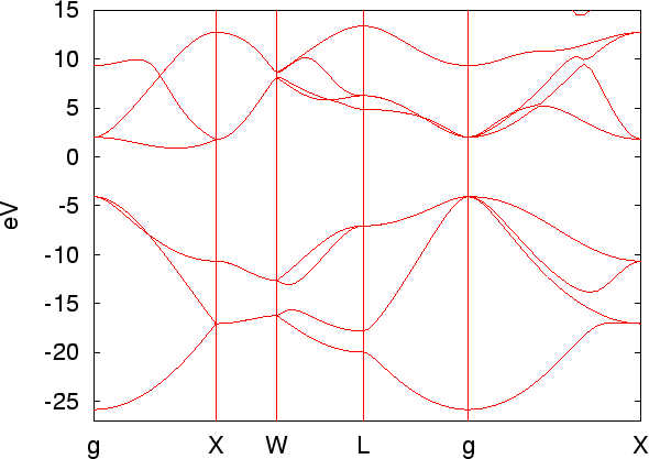
Figure 12 shows the band dispersion of carbon diamond, generated by the above procedure, while the range of y-axis was changed in the file cdia.GNUBAND. It is also noted that the chemical potential is automatically shifted to the origin of energy.

A problem in drawing of the band dispersion is how to choose a unit cell used in calculating of the band dispersion. Often, the unit cell used in calculating of the band dispersion is different from that used in the definition of the periodic system. In such a case you need to define the unit cell used in calculating of the band dispersion by the keyword 'Band.KPath.UnitCell'. If you define 'Band.KPath.UnitCell', the reciprocal lattice vectors for the calculation of the band dispersion are calculated by the unit vectors specified in 'Band.KPath.UnitCell'. If you do not define 'Band.KPath.UnitCell', the reciprocal lattice vectors, which are calculated by the unit vectors specified in 'Atoms.UnitVectors' is employed for the calculation of the band dispersion. In case of fcc, bcc, base centered cubic, and trigonal cells, the reciprocal lattice vectors for the calculation of the band dispersion should be specified using the keyword 'Band.KPath.UnitCell' based on the consuetude in the band calculations.