Exact exchange by a range-separated exchange hole
Masayuki Toyoda* and Taisuke Ozaki
Research Center for Integrated Science (RCIS),
Japan Advanced Institute of Science and Technology (JAIST),
1-1 Asahidai, Nomi, Ishikawa 923-1292, Japan.
April 1, 2011
This is the author version of article published as:
M. Toyoda and T. Ozaki, Phys. Rev. A 83, 032515 (2011).
Copyright 2011 by the American Physics Socienty.
Abstract
An approximation to the exchange-hole density is proposed for the
evaluation of the exact exchange energy in electronic structure
calculations within the density-functional theory and the Kohn-Sham
scheme.Based on the localized nature of density matrix, the exchange
hole is divided into the short-range (SR) and long-range (LR) parts
by using an adequate filter function, where the LR part is deduced by
matching of moments with the exactly calculated SR counterpart, ensuring
the correct asymptotic

behavior
of the exchange potential. With this division, the time-consuming
integration is truncated at a certain interaction range, largely
reducing the computation cost. The total energies, exchange energies,
exchange potentials, and eigenvalues of the highest-occupied orbitals
are calculated for the noble-gas atoms. The close agreement of the
results with the exact values suggests the validity of the approximation.
The density-functional theory
[1]
in the formulation by Kohn, Sham, and Levy
[2,
3] (KS-DFT) is a methodology that is
now recognized as one of the most powerful tools to investigate the
electronic structures of atoms, molecules and solids. The high
computational efficiency is afforded by transforming the problem of
interacting electrons to a single-body problem of noninteracting
electrons placed in an effective potential. Therefore, the central
problem lies in the in which to describe the electronic exchange and
correlation by the effective potential. The local-density approximation
(LDA) [2] describes it as a local
potential that is derived from the exchange and correlation energy of a
uniform electron gas. In the generalized gradient approximation (GGA)
[4,
5,
6], a semilocal potential is used where the
electronic density gradient is also taken into account. The local and
semilocal effective potentials provide a well-balanced compromise
between reliability and feasibility and are, thus, used routinely in the
fields of quantum chemistry, solid-state physics, and biophysics.
The KS-DFT methods with LDA and GGA are, however, also known for
systematic errors such as the significant underestimation of the
band-gap energy of semiconductors and insulators. The failure of the
semilocal approximation is manifested by the incomplete cancellation of
the self-Hartree energy for each orbital, known as the self-interaction
error (SIE), and the incorrect asymptotic decay of the
exchange-correlation potential. Since it is primarily caused by the poor
description of the exchange interaction, the error is remedied by using
the exact exchange (EXX). There have been several such approaches
including the hybrid functional methods
[7,
8,
9,
10] where a fraction (typically,
 ) of EXX are admixed with the
semilocal exchange and the range-separated exchange methods
[11,
12,
13,
14] where either the short-range (SR)
or long-range (LR) part of EXX is combined with the semilocal
counterpart.
) of EXX are admixed with the
semilocal exchange and the range-separated exchange methods
[11,
12,
13,
14] where either the short-range (SR)
or long-range (LR) part of EXX is combined with the semilocal
counterpart.
The high computation cost required for the evaluation of EXX is an
obvious drawback of the hybrid methods. The scaling of the computation
in the canonical way is
 where
where
 is a measure of the system size. Although it can be reduced to
 in a local-basis implementation
[15], it is still higher than the
in a local-basis implementation
[15], it is still higher than the
 scaling of the semilocal exchange. A further reduction of the scaling
may be attained by modifying the exchange interaction into the
screened exchange interaction by multiplying an exponentially
decaying factor to the Coulomb operator. Among the above-mentioned
methods, this approach is employed in the screened hybrid functional
method [10] and the screened-exchange
LDA method [12,
14]. Not only being advantageous in
terms of computation time, this technique is as well found to mimic a
part of the correlation effects by screening out the LR part of exchange
and to improve the results for several quantities in metals and
semiconductors. However, the other groups
[13,
16,
17,
18] take the opposite idea where
the LR part of EXX (or the exchange-correlation calculated by a post
Hartree-Fock (HF) method) is combined with the SR part of a semilocal
exchange-correlation, claiming the importance of the LR asymptotic tail
of the exchange potential. A way to somehow recover the correct
tail of the screened-exchange potential, therefore, seems to be
advantageous in both the physical and computational point of views.
scaling of the semilocal exchange. A further reduction of the scaling
may be attained by modifying the exchange interaction into the
screened exchange interaction by multiplying an exponentially
decaying factor to the Coulomb operator. Among the above-mentioned
methods, this approach is employed in the screened hybrid functional
method [10] and the screened-exchange
LDA method [12,
14]. Not only being advantageous in
terms of computation time, this technique is as well found to mimic a
part of the correlation effects by screening out the LR part of exchange
and to improve the results for several quantities in metals and
semiconductors. However, the other groups
[13,
16,
17,
18] take the opposite idea where
the LR part of EXX (or the exchange-correlation calculated by a post
Hartree-Fock (HF) method) is combined with the SR part of a semilocal
exchange-correlation, claiming the importance of the LR asymptotic tail
of the exchange potential. A way to somehow recover the correct
tail of the screened-exchange potential, therefore, seems to be
advantageous in both the physical and computational point of views.
In this paper, a scheme to calculate EXX is proposed with our goal to
achieve high computational efficiency comparable to the computation of
the semilocal exchange.
Although the idea of the range-separated exchange is utilized, neither the SR
nor LR part is screened out.
The fundamental idea behind the presented scheme is the general nature
of electrons in materials that the electronic structure is much less
sensitive to a change of an external potential in a far-away region.
This principle is known as nearsightedness [19],
forming the basis of linear-scaling DFT methods [20].
Our ansatz is as follows: the SR part of the exchange potential possesses most of
the physical significance and, thus, the LR part is easily estimated by
referring the SR counterpart.
This idea may enable us to develop an exchange functional for KS-DFT
calculations where the exact properties of EXX are fulfilled, such
as the cancellation of SIE and the correct asymptotic behavior of the
exchange potential, with computation cost.
This paper is organized as follows.
In Sec. II, the detailed formulation of the scheme is presented.
In Sec. III, the computation results for noble-gas atoms are shown
and the manner in which the ansatz works for atomic systems is discussed.
Finally, a summary is given in Sec. IV.
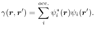
In KS-DFT, EXX for a spin channel is given, in atomic units (
 ),
as follows:
),
as follows:
 |
(1) |
where
 is the
  -th KS orbital and the summation is taken over
all the occupied orbitals.
This is not an explicit functional of the total charge density
-th KS orbital and the summation is taken over
all the occupied orbitals.
This is not an explicit functional of the total charge density
 but
of the first-order reduced density matrix (1-RDM)
but
of the first-order reduced density matrix (1-RDM)
 |
(2) |
The exchange energy (1) is also expressible in the following form:
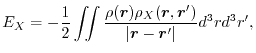 |
(3) |
where
 is the exchange hole density
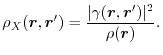 |
(4) |
As in the case of the range-separated exchange methods, the exchange hole is
divided into the SR and LR parts as follows:
 |
(5) |
where  is a function of
 which is unity at
  and decreases rapidly (exponentially, in general)
as
and decreases rapidly (exponentially, in general)
as  increases, approaching to zero at
 .
Therefore, the first and second terms of right-hand side (r.h.s) in Eq. (5)
correspond to the SR and LR parts of the exchange hole, respectively.
.
Therefore, the first and second terms of right-hand side (r.h.s) in Eq. (5)
correspond to the SR and LR parts of the exchange hole, respectively.
Here, we estimate the LR part by referring the SR part.
A qualitative support to this idea is given by the fact that the 1-RDM in
materials shows rapid decay as
 where the exponent is
 (small gap) or
 (large gap) in an insulator with direct gap energy
  , and
, and
 (low temperature)
or
(low temperature)
or
 (high temperature) in a metal with electronic temperature
  [21,22].
Under the idea, the LR part is replaced by an analytic function
[21,22].
Under the idea, the LR part is replaced by an analytic function
 which models the spherically averaged exchange hole
where
which models the spherically averaged exchange hole
where
 is a composite parameter determined self-consistently at each point of
  in space.
Note that the spherical average does not lack mathematical rigor because
of the isotropic nature of the Coulomb interaction.
Our exchange hole is, therefore,
in space.
Note that the spherical average does not lack mathematical rigor because
of the isotropic nature of the Coulomb interaction.
Our exchange hole is, therefore,
 |
(6) |
which should fulfill the conditions that an exact exchange hole does,
such as the non-negativity and the unit normalization
 |
(7) |
By substituting Eq. (6) in Eq. (3), the exchange energy is given as
 |
(8) |
where
 |
(9) |
The decaying function in Eq. (8) enables one to terminate
the numerical integration at a finite interaction length
 ,
which reduces the scaling of the computation.
,
which reduces the scaling of the computation.
So far, the scheme is introduced without defining the decaying function
and the model exchange hole function
 .
In the preceding works, two types of decaying functions have been used.
One is the Thomas-Fermi- (TF-) type screening function [11],
.
In the preceding works, two types of decaying functions have been used.
One is the Thomas-Fermi- (TF-) type screening function [11],
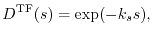 |
(10) |
where  is the Thomas-Fermi wavevector [23].
This is of the same shape as Yukawa's short-range nuclear force.
The other type is called the erf screening [16]:
is the Thomas-Fermi wavevector [23].
This is of the same shape as Yukawa's short-range nuclear force.
The other type is called the erf screening [16]:
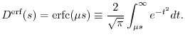 |
(11) |
As a variation of the erf screening, Toulouse et al. have recently
proposed another function called erfgau interaction [17].
As the first test, we choose
 for our decaying function.
The parameter
for our decaying function.
The parameter  determines the range in which the SR and LR parts are separated.
For the model exchange hole, the following form is used
determines the range in which the SR and LR parts are separated.
For the model exchange hole, the following form is used
![$\displaystyle f_H(a, b, s)
=
\frac{a}{16 \pi b s}
\left[ (a\vert b-s\vert+1)...
...-s\vert) \right.
\left.
-(a\vert b+s\vert+1)\exp(-a\vert b+s\vert) \right]
.$](img55.png) |
(12) |
This is analytically derived from the  wave function of a hydrogenic atom and
was previously used by Becke and Roussel [24]
to describe the exchange hole in a meta-GGA method.
By construction, the function (12) satisfies the exact conditions for
an exchange hole: it has always a non-negative value and the norm is
unity throughout its domain (
wave function of a hydrogenic atom and
was previously used by Becke and Roussel [24]
to describe the exchange hole in a meta-GGA method.
By construction, the function (12) satisfies the exact conditions for
an exchange hole: it has always a non-negative value and the norm is
unity throughout its domain ( ,
,  , and
, and  ).
With the choice, the exchange energy [Eq. (3)] and the LR energy density [Eq. (9)]
have the following explicit forms:
).
With the choice, the exchange energy [Eq. (3)] and the LR energy density [Eq. (9)]
have the following explicit forms:
 |
(13) |
and
respectively, where  and
and  .
.
The model parameters  and
and  are determined by matching moments of
the exchange hole.
The
are determined by matching moments of
the exchange hole.
The  -th moment of the exactly calculated SR part is
while that of the corresponding SR part of the model exchange hole is
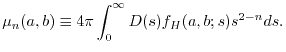 |
(16) |
The conditions appropriate for determination of the parameters might be
 |
(17) |
and
 |
(18) |
which physically mean the normalization of the hole (7) and
the agreement of the SR exchange potential, respectively.
The conditions (17) and (18) must and can be met
simultaneously if the model function has enough flexibility to reproduce
the exact hole.
In practice, however, there is no guarantee for the existence of and
that satisfies both the requirements for a given model function.
In fact, with Eq. (12), we found it impossible to find
and to satisfy both requirements simultaneously for a certain range
of values of
 and
and
 ).
Therefore, we search and , which give
).
Therefore, we search and , which give  most close to
  instead of the condition (18), while keeping the other condition
(17) satisfied.
This search is achieved by using the Lagrange multipliers.
The Lagrangian is
instead of the condition (18), while keeping the other condition
(17) satisfied.
This search is achieved by using the Lagrange multipliers.
The Lagrangian is
![$\displaystyle {\cal L}(a, b)
=
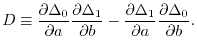
\left[ \Delta_1(a,b) \right]^2 + \lambda \Delta_0(a,b) + P(b)
,$](img77.png) |
(19) |
where  is the relative difference between the exact moment and
the model moment
is the relative difference between the exact moment and
the model moment
 |
 |
(20) |
and
 |
(21) |
is a penalty function, with an arbitrary constant  ,
which is introduced to prevent from being too small due to
a technical reason that some of the
analytic expressions such as Eq. (14) become
numerically unstable when approaches to zero.
At the stationary point of
,
which is introduced to prevent from being too small due to
a technical reason that some of the
analytic expressions such as Eq. (14) become
numerically unstable when approaches to zero.
At the stationary point of  , three conditions are obtained by
differentiating with respect to , , and
, three conditions are obtained by
differentiating with respect to , , and  .
One of them is, of course, the condition (17).
By erasing from the remaining two conditions, the following
condition is obtained:
.
One of them is, of course, the condition (17).
By erasing from the remaining two conditions, the following
condition is obtained:
 |
(22) |
where
 |
(23) |
For a fixed value of , the model function (12) is a monotonic
function of .
It is thus easy to find which satisfies the requirement (17)
for given by using a simple search algorithm such as the bisection search.
Then, since now can be treated as a bound variable, it is also
straightforward to find which satisfies the remaining requirement (22).
Therefore, the determination process is a tractable task.
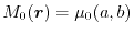
Computation of the moments is also not time-consuming for the
following reason:
Calculating  over the whole space is computationally
similar with taking an integral over of Eq. (15),
which leads to almost the same expression as the first term of Eq. (8).
Therefore, it can be performed by applying conventional techniques for
calculating EXX, for example, by calculating the electron-repulsion
integrals of the Gaussian basis set [25] or of a
numerically defined localized basis set [15].
The computation is actually not heavier than the
calculation of the energy (8) itself.
over the whole space is computationally
similar with taking an integral over of Eq. (15),
which leads to almost the same expression as the first term of Eq. (8).
Therefore, it can be performed by applying conventional techniques for
calculating EXX, for example, by calculating the electron-repulsion
integrals of the Gaussian basis set [25] or of a
numerically defined localized basis set [15].
The computation is actually not heavier than the
calculation of the energy (8) itself.
The effective potential for the KS equations that corresponds to the
exchange energy (13) is obtained by taking the functional
derivatives with respect to variations of the KS orbitals.
The functional derivatives in the present scheme are well-defined
except for the model parameters and .
Since they have to be optimized numerically, there is no analytic
relation between the parameters and the orbital wave functions.
However, since the conditions (17) and (22)
are assumed to be rigorously satisfied, the conditions must also be
stationary against the variations and, thus, the following equations
are obtained:
They are arranged in the following algebraic representation,
 |
(26) |
where  and
and  are
are  matrices with the matrix elements
 |
 |
(27) |
 |
 |
(28) |
 |
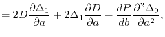 |
(29) |
 |
 |
(30) |
 |
 |
(31) |
 |
 |
(32) |
and
 .
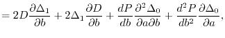
Since the variation of
.
Since the variation of  and is well defined, the variation of the parameters
can be analytically obtained as follows:
and is well defined, the variation of the parameters
can be analytically obtained as follows:
 |
(33) |
Finally, the functional derivative of Eq. (13) is explicitly given as
where
and  is the matrix element of
 .
The first term of RHS in Eq. (34) is a
Hartree-Fock-type non-local potential and, thus, is dealt with by
the Fock matrix of the Roothann equation in terms of a
basis set expansion where the Coulomb operator is replaced with
.
The first term of RHS in Eq. (34) is a
Hartree-Fock-type non-local potential and, thus, is dealt with by
the Fock matrix of the Roothann equation in terms of a
basis set expansion where the Coulomb operator is replaced with
 |
(37) |
While, the second term is a semilocal potential and treated in the
same way as the LDA potential.
The derivatives with respect to the atomic nuclear positions are
often required to calculate the force acting on the atoms for
molecular dynamic simulations.
The derivatives are also analytically obtained by using the
relation of Eq. (33).
The importance of using EXX lies mainly in the fact that the self-exchange
energy for each KS orbital exactly cancels the corresponding self-Hartree energy.
In this scheme,
exchange energy for -th orbital is
where
 is the orbital charge density.
This includes both the self- and mutual-exchange energy. In the sum in the first term, the
is the orbital charge density.
This includes both the self- and mutual-exchange energy. In the sum in the first term, the  term describes the SR part of the self-exchange energy while the other
  terms are the SR part of the mutual-exchange energy. In the second term, the separation of the self-exchange from the mutual-exchange is not clear.
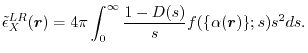
The remaining term is characterized by the factor
terms are the SR part of the mutual-exchange energy. In the second term, the separation of the self-exchange from the mutual-exchange is not clear.
The remaining term is characterized by the factor
 |
(39) |
which is the difference between the non-local orbital density and 1-RDM
weighted by the orbital density.
It vanishes after taking summation over orbitals.
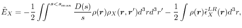
In one-electron systems, such as a hydrogen atom, the first and second terms are the correct self-exchange energy and the third term vanishes. For many electron-systems, although the first term correctly cancels the SR part of the self-Hartree energy, the second term might include the LR part of the self-exchange energy and the third term does not vanish.
However, since SIE is significant for a localized orbital and the difference
(39) is small when and  are close to each
other, it is expected that the LR part of the self-exchange and
the difference [Eq. (39)] can be negligible and, therefore,
that SIE is nearly completely canceled in the present method.
are close to each
other, it is expected that the LR part of the self-exchange and
the difference [Eq. (39)] can be negligible and, therefore,
that SIE is nearly completely canceled in the present method.
The presented method has been implemented in our in-house program for
electronic structure calculations of atomic systems based on the
real-space finite-element method [26].
The advantage of the program is that all the integrations are performed
analytically except for those for the exchange-correlation energy.
For the exchange-correlation energy, the integration is performed by
interpolating the charge density and the exchange-correlation potential
with a set of finite-element basis functions.
Therefore, the numerical error is determined solely by the
interval of the radial grid points.
In the following results, we have confirmed the convergence of the
energy at least to the number of digits shown in the tables.
The deviations from the exact values are thus directly attributed to
the approximation of the presented method.
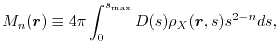
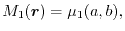
In Fig. 1, the exchange-hole density of a neon atom
is plotted around a reference point at  a.u. away from the
nucleus.
The profile consists of a sharp peak from the core electrons and a
broad feature from the valence electrons.
The exchange hole in this method [Eq. (6)] is plotted
by the dashed line where the separation parameter is chosen to be
a.u. away from the
nucleus.
The profile consists of a sharp peak from the core electrons and a
broad feature from the valence electrons.
The exchange hole in this method [Eq. (6)] is plotted
by the dashed line where the separation parameter is chosen to be
 .
The dotted line shows the SR part of the hole.
It is clearly shown that the exact hole is localized within
.
The dotted line shows the SR part of the hole.
It is clearly shown that the exact hole is localized within  a.u.
and thus described well almost only by the SR part.
a.u.
and thus described well almost only by the SR part.
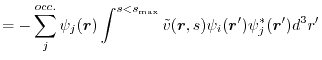
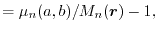
In Fig. 2, the exchange-hole density of an argon atom
is plotted around a reference point at  a.u. away from the nucleus.
In this case, the profile becomes more complicated, reflecting the atomic
shell structure.
Although the shape is rather smeared out [27], the three dominant
peaks are still well captured by this method.
a.u. away from the nucleus.
In this case, the profile becomes more complicated, reflecting the atomic
shell structure.
Although the shape is rather smeared out [27], the three dominant
peaks are still well captured by this method.
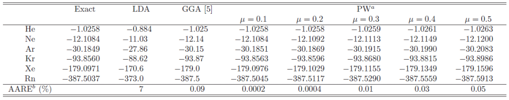
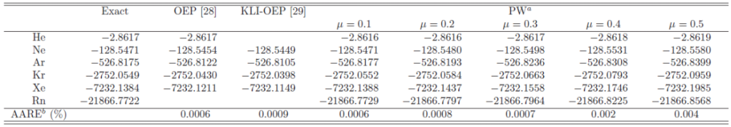
Table 1:
|
In Table 1, the exchange energy of the noble-gas atoms calculated
by the present method with various values of the parameter are
summarized and compared with the LDA, GGA, and exact results.
All the energies are calculated with the exact wave function obtained
by the HF calculations.
The average absolute relative errors (AARE) from the exact values are listed in the bottom line. The values obtained by the present work (PW) are arranged in columns with different values of .
For smaller values of , the presented method yields quite accurate
exchange energies with error in order of 1 mili-hartree or even less than that.
The error systematically increases as increases.
With
 , the error is almost in the same
order as the GGA results.
Note that the GGA exchange energy is also acceptably accurate because
the enhancement factor was often constructed to reproduce the exact
exchange energy of the noble-gas atoms.
The problem of the GGA exchange is actually in the description of the
potential.
Since the presented method can also yield an accurate potential
as shown later, even the method with
performs much better than GGA.
, the error is almost in the same
order as the GGA results.
Note that the GGA exchange energy is also acceptably accurate because
the enhancement factor was often constructed to reproduce the exact
exchange energy of the noble-gas atoms.
The problem of the GGA exchange is actually in the description of the
potential.
Since the presented method can also yield an accurate potential
as shown later, even the method with
performs much better than GGA.
Table 2:
|
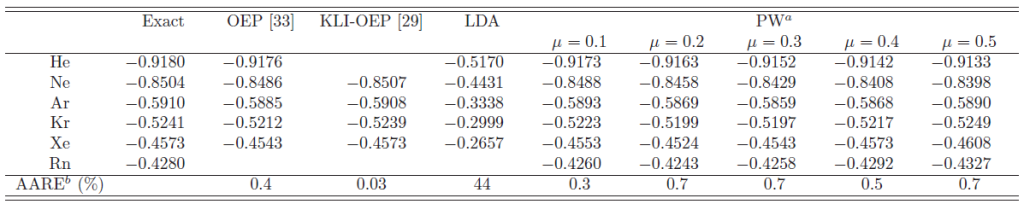
In Table 2, the total energy of the noble-gas atoms in the
exchange-only calculations is summarized and compared with the values
calculated with the optimized effective potentials (OEP) [30,31]
, as well as the exact value by the HF method.
The OEP method has been used to evaluate EXX in the KS-DFT method with
a local effective potential.
Although it has been shown that the exact local exchange potential does not
exist for the ground state of typical atoms [32],
the OEP methods can give very accurate energies as shown in Table 2.
The presented method with smaller values of also yields the total energy
close to the exact value, while, for larger values of , it becomes worse
than the OEP method.
Interestingly, there seems to be a general tendency that the total energy
by the presented method becomes lower as increases, while
the OEP values are always higher than the exact value.
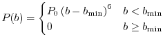
Finally, the question ought to be considered as to whether the present scheme
can successfully reproduce the LR asymptotic tail of the exchange
potential as expected.
In Fig. 3, the calculated exchange potential of a
helium atom is shown.
The potential is defined here as the Coulomb potential generated by the
exchange hole
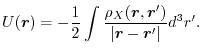 |
(40) |
The LDA potential shows the well-known difference from the exact potential.
For example, the asymptotic tail approaches to zero much faster than the
exact tail.
The GGA potential not only shows no improvement in the tail, but also has
an erroneous divergence at the origin.
On the contrary, our method successfully reproduce the exact
exchange potential.
Table 3:
|
Note that the plotted potential (40) is different from the
effective exchange potentials (34) appearing in the
KS equations.
To see that the effective potential (34) also has
the correct shape, the single-particle eigenvalue of the highest-occupied state
(HOS) is calculated and summarized in Table 3.
This serves as a simple but sensitive test as to whether the exchange potential
has the correct asymptotic tail because it determines the tail of the HOS charge density.
The LDA eigenvalue is much too high as commonly known, showing
that it has a completely wrong potential at the asymptotic region.
The presented method, on the other hand, can calculate reasonably accurate
eigenvalues with error less than 1%.
We have shown that the presented method can reproduce accurate exact exchange
energy and potential, and also that the degree of the approximation is systematically controlled
by the separation parameter from the level of GGA (
 )
to the level of OEP (
)
to the level of OEP (
 ) or to even higher than that.
This result would at least partly validate our ansatz that the LR part of the
exchange energy can be well described by referring the corresponding SR part.
The remaining question is how much the computation load can be reduced
by the presented method with the typical values of .
As a rough estimation, the effective range of the screening of
is given as
) or to even higher than that.
This result would at least partly validate our ansatz that the LR part of the
exchange energy can be well described by referring the corresponding SR part.
The remaining question is how much the computation load can be reduced
by the presented method with the typical values of .
As a rough estimation, the effective range of the screening of
is given as
 |
(41) |
The values are
 ,
,  , and
, and
 at
at  ,
,  , and
, and
 , respectively.
In actual calculations of the screened hybrid functional method [10],
for example, the exchange energy contribution in a metallic carbon nanotube is
reported to be converged at around
, respectively.
In actual calculations of the screened hybrid functional method [10],
for example, the exchange energy contribution in a metallic carbon nanotube is
reported to be converged at around
 when the screening
function
with
when the screening
function
with
 is used.
We, therefore, expect that, by using the medium value
is used.
We, therefore, expect that, by using the medium value
 ,
a reasonably accurate EXX can be calculated where the integrations are
terminated at
,
a reasonably accurate EXX can be calculated where the integrations are
terminated at
 .
A quantitative study is in progress where the presented method is implemented
in a conventional DFT program and applied to molecules and solids.
.
A quantitative study is in progress where the presented method is implemented
in a conventional DFT program and applied to molecules and solids.
We have presented a scheme to calculate EXX with
computational scaling by truncating the numerical integrations,
while the correct asymptotic tail of the exchange potential
is well reproduced by an approximation to the tail of the exchange-hole density.
The numerical calculations for the noble-gas atoms show that
the presented scheme can provide accurate exchange energies.
The method is based on a fundamental idea that the LR behavior
of the interaction should somehow be extrapolated by referring the
information obtained from the corresponding SR part due to the
localized nature of 1-RDM of electrons.
This idea should also be applicable for other methodologies
based on 1-RDM, e.g. the reduced-density-matrix functional
method and post HF methods.
The low computational cost is advantageous especially for the
large scale calculations and the present method can be immediately
applied in the framework of the hybrid functional method or the
range-separated EXX method.
It would be, however, more challenging to search for a scheme with
low computational cost based on the same idea for the correlation
functional that is compatible with EXX.
This work was partly supported by CREST-JST, the Next Generation Super
Computing Project, Nanoscience Program, MEXT, Japan, and ``Materials
Design through Computics: Complex Correlation and Non-Equilibrium
Dynamics'' A Grant in Aid for Scientific Research on Innovative Areas
MEXT, Japan.
- P. Hohenberg and W. Kohn, Phys. Rev. 136, B864 (1964).
- W. Kohn and L. J. Sham, Phys. Rev. 140, A1133 (1965).
- M. Levy, Proc. Natl. Acad. Sci. USA 76, 6062 (1979).
- J. P. Perdew, K. Burke, and M. Ernzerhof, Phys. Rev. Lett. 77, 3865 (1996).
- A. D. Becke, Phys. Rev. A 38, 3098 (1988).
- J. P. Perdew and Y. Wang, Phys. Rev. B 45, 13244 (1992).
- A. D. Becke, J. Chem. Phys. 98, 1372 (1993).
- J. P. Perdew, J. P. Perdew, M. Ernzerhof, and K. Burke, J. Chem. Phys. 105, 9982 (1996).
- C. Adamo and V. Barone, J. Chem. Phys. 110, 6158 (1999).
- J. Heyd, G. E. Scuseria, and M. Ernzerhof, J. Chem. Phys. 118, 8207 (2003).
- D. M. Bylander and L. Kleinman, Phys. Rev. B 41, 7868 (1990).
- A. Seidl, A. Görling, P. Vogl, J. A. Majewski, and M. Levy, Phys. Rev. B 53, 3764 (1996).
- H. Iikura, T. Tsuneda, T. Yanai, and K. Hirao, J. Chem. Phys. 115, 3540 (2001).
- S. J. Clark and J. Robertson, Phys. Rev. B 82, 085208 (2010).
- M. Toyoda and T. Ozaki, J. Chem. Phys 130, 124114 (2009).
- T. Leininger, H. Stoll, H.-J. Werner, and A. Savin, Chem. Phys. Lett. 275, 151 (1997).
- J. Toulouse, F. Colonna, and A. Savin, Phys. Rev. A 70, 062505 (2004).
- J. Toulouse, P. Gori-Giorgi, and A. Savin, Int. J. Quantum Chem. 106, 2026 (2006).
- W. Kohn, Phys. Rev. Lett. 76, 3168 (1996).
- S. Goedecker, Rev. Mod. Phys. 71, 1085 (1999).
- S. Ismail-Beigi and T. A. Arias, Phys. Rev. Lett. 82, 2127 (1999).
- S. Goedecker, Phys. Rev. B 58, 3501 (1998).
- W. A. Harrison, Solid State Theory (McGraw-Hill, New York, 1970).
- A. D. Becke and M. R. Roussel, Phys. Rev. A 39, 3761 (1989).
- S. H. H. Taketa and K. O-ohata, J. Phys. Soc. Jpn. 21, 2313 (1966).
- T. Ozaki and M. Toyoda, Comput. Phys. Commun. (in press).
- The smearing shows the limitation of the model function Eq. (12) not to have a multiple-peak structure because it is derived from a node-less orbital.
- Y. Wang, J. P. Perdew, J. A. Chevary, L. D. Macdonald, and S. H. Vosko, Phys. Rev. A 41, 78 (1990).
- J. B. Krieger, Y. Li, and G. J. Iafrate, Phys. Rev. A 45, 101 (1992).
- R. T. Sharp and G. K. Horton, Phys. Rev. 90, 317 (1953).
- J. D. Talman and W. F. Shadwick, Phys. Rev. A 14, 36 (1976).
- R. K. Nesbet and R. Colle, Phys. Rev. A 61, 012503 (1999).
- Y. Li, J. B. Krieger, J. A. Chevary, and S. H. Vosko, Phys. Rev. A 43, 5121 (1991).
This document was generated using the
LaTeX2HTML translator Version 2002-2-1 (1.71)
Copyright © 1993, 1994, 1995, 1996,
Nikos Drakos,
Computer Based Learning Unit, University of Leeds.
Copyright © 1997, 1998, 1999,
Ross Moore,
Mathematics Department, Macquarie University, Sydney.
TOYODA Masayuki
2011-04-01
![$\displaystyle \hspace{8em} +\iint d^3r d^3r' D(s)\left( \alpha(\vec r) + \frac{...
...o(\vec r)}\gamma(\vec r, \vec r') - \psi^*_i(\vec r) \psi_i(\vec r') \right]
,$](img123.png)
![$\displaystyle \hspace{12em}
\left. \left. \vphantom{\int}
- \left( x^2-1+xy \right) \mathrm{erfc}(x+y) e^{xy} \right] \right\}
,$](img63.png)