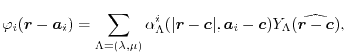
LIBERI: Library for Numerical Evaluation of Electron-Repulsion Integrals
Masayuki Toyoda* and Taisuke Ozaki
Research Center for Integrated Science,
Japan Advanced Institute of Science and Technology,
1-1, Asahidai, Nomi, Ishikawa 932-1292, Japan
Copyright 2010 Elsevier B.V.
This article is provided by the author for the reader's personal use only.
Any other use requires prior permission of the author and Elsevier B.V.
NOTICE: This is the authorÅfs version of a work accepted for publication by Elsevier.
Changes resulting from the publishing process, including peer review, editing,
corrections, structural formatting and other quality control mechanisms, may
not be reflected in this document. Changes may have been made to this work
since it was submitted for publication. A definitive version was subsequently
published in Computer Physics Communications 181, 1455-1463 (2010),
DOI: 10.1016/j.cpc.2010.03.019 and may be found at
http://dx.doi.org/10.1016/j.cpc.2010.03.019.
*Corresponding author:
Masayuki Toyoda,
Postal Address: Research Center for Integrated Science,
Japan Advanced Institute of Science and Technology,
1-1, Asahidai, Nomi, Ishikawa 932-1292, Japan.
Phone: +81-761-51-1987
E-mail: m-toyoda (at) jaist.ac.jp.
Abstract
We provide a C library, called LIBERI, for numerical evaluation of
four-center electron repulsion integrals, based on successive
reduction of integral dimension by using Fourier transforms.
LIBERI enables us to compute the integrals for numerically defined
basis functions within  Hartree accuracy as well as their
derivatives with respect to the atomic nuclear positions.
Damping of the Coulomb interaction can also be imposed to take
account of screening effect.
Hartree accuracy as well as their
derivatives with respect to the atomic nuclear positions.
Damping of the Coulomb interaction can also be imposed to take
account of screening effect.
Keywords: Ab initio calculations, Exchange interactions, Exchange-correlation functionals
PACS: 31.15A-; 71.70Gm; 31.15eg
PROGRAM SUMMARY
Manuscript Title: LIBERI: Library for Numerical Evaluation of
Electron-Repulsion Integrals
Authors: M. Toyoda and T. Ozaki
Program Title: LIBERI
Journal Reference:
Catalogue identifier:
Licensing provisions: none
Programming language: C
Computer: all
Operating system: any Unix-like system
RAM: 5 - 10 MB
Keywords: Ab initio calculations, Exchange interactions,
Exchange-correlation functionals
PACS: 31.15A-; 71.70Gm; 31.15eg
Classification: 7.4 Electronic Structure
External routines/libraries: LAPACK, FFTW3
Nature of problem: Numerical evaluation of four-center
electron-rupulsion integrals
Solution method:
Four-center electron-repulsion integals are computed for given
basis function set, based on successive reduction of integral
dimension using Fourier transform.
Running time: 0.5 sec for the demo program supplied with the
package
Introduction
The efficient and accurate evaluation of the four-center
electron-repulsion integrals (ERIs) is an essential task in
computational studies of the electronic structures of
molecules and solids.
For given basis functions
 ,
,
 ,
,
 and
and
 located at
 ,
,  ,
,  and
and  , respectively,
ERI is defined as,
, respectively,
ERI is defined as,
Conventionally, Gaussian-type orbitals (GTOs) are used for the basis
functions
 in Eq. (1).
This is due to the fact that with the GTOs the integrals can be
evaluated quite easily [1].
Improvements in the numerical methods for the evaluation of ERIs for
GTOs have been made for more than a half
century [2,3,4,5].
Although GTOs are convenient for mathematical operations, they are not
suitable to describe atomic wave functions because they do not satisfy
two important conditions for solutions of the atomic Schrödinger
equation, namely the exponential decay at long range and the cusp at
the origin.
This problem can be overcome by taking contractions of GTOs to mimic
realistic atomic wave functions with the appropriate nuclear cusp
behaviors.
However, the increase in the number of basis functions by the
contractions causes a more significant increase in the number of
required integrals to be computed.
in Eq. (1).
This is due to the fact that with the GTOs the integrals can be
evaluated quite easily [1].
Improvements in the numerical methods for the evaluation of ERIs for
GTOs have been made for more than a half
century [2,3,4,5].
Although GTOs are convenient for mathematical operations, they are not
suitable to describe atomic wave functions because they do not satisfy
two important conditions for solutions of the atomic Schrödinger
equation, namely the exponential decay at long range and the cusp at
the origin.
This problem can be overcome by taking contractions of GTOs to mimic
realistic atomic wave functions with the appropriate nuclear cusp
behaviors.
However, the increase in the number of basis functions by the
contractions causes a more significant increase in the number of
required integrals to be computed.
An alternative approach to evaluate ERIs has been developed by
Talman [6] for general types of basis functions where the
radial part is defined numerically on a radial mesh.
In his paper, the multicenter integrals including ERIs are evaluated
for Slater-type orbital (STO) basis.
In our previous paper [7], we have implemented
Talman's approach in a program code and evaluated the ERIs for the
strictly localized pseudo-atomic orbitals (PAOs) [8] which
are obtained by solving Schrödinger-like equations with confinement
conditions.
The PAO basis sets are suitable for linear scaling method and thus for
large scale ab initio calculations.
We have also presented some extension to Talman's approach such as the
formulation of the derivatives of ERIs with respect to the nuclear
positions and the modification of the equations to take the screening
effect into account by making the Coulomb interaction short-range.
In the preset paper, we extract the relevant subroutines from our
program code, pack them up, and present it as an independent library
named LIBERI (LIBrary for numerical evaluation of ERIs).
In Section 2, the basic equations of LIBERI are briefly reviewed.
More detailed topics on the numerical techniques, especially for the
spherical Bessel transform are presented in Section 3.
Instruction how to compile and use LIBERI is provided in the following
sections.
In Section 6, we estimate required computation time in actual
calculations.
Formulation
In this section, the equations used in LIBERI are outlined.
For the detailed derivations, we refer readers to the original work by
Talman [6] as well as our previous
article [7].
What LIBERI does is to compute Eq. (1) for given basis
functions.
Each basis function is decomposed into its radial and angular
components,
 |
(2) |
where
 is the spherical harmonic function for a given
angular momentum
is the spherical harmonic function for a given
angular momentum
 .
The radial part
.
The radial part  is an arbitrarily shaped (but localized in a
usual sense) function which is numerically defined on a radial mesh.
is an arbitrarily shaped (but localized in a
usual sense) function which is numerically defined on a radial mesh.
The calculation of a ERI consists of two distinct parts.
The first step is to calculate a function which describes the overlap
of
and
, and another one for
and
.
Then, the second part evaluates the ERI in the same manner as the
calculation of the electrostatic energy of two electrons whose charge
distribution is described by the overlap functions.
Let us define the overlap function
 which is defined
for
and
, and
which is defined
for
and
, and
 for
and
,
for
and
,
where  and
and  are arbitrarily chosen centers.
Obviously, should be located at somewhere between
and , and at somewhere between and
.
We will discuss in Section 3.3 on how to determine the
positions of and in actual calculations.
In order to calculate the overlap functions, the centers of the basis
functions should be translated, which means, for example,
located at has to be described in a
spherical coordinate centered at .
Such translation is described by using Löwdin's
are arbitrarily chosen centers.
Obviously, should be located at somewhere between
and , and at somewhere between and
.
We will discuss in Section 3.3 on how to determine the
positions of and in actual calculations.
In order to calculate the overlap functions, the centers of the basis
functions should be translated, which means, for example,
located at has to be described in a
spherical coordinate centered at .
Such translation is described by using Löwdin's
 -functions [9] as follows:
Here,
 is given by multiplying a
phase shift which corresponds to the constant spatial shift
is given by multiplying a
phase shift which corresponds to the constant spatial shift  with
the basis function in Fourier space and by transforming it back to
real space
with
the basis function in Fourier space and by transforming it back to
real space
where  is the spherical Bessel function of the first kind
and
is the spherical Bessel function of the first kind
and
 is the Gaunt coefficients defined by
 |
(9) |
The translation of the expansion center in Eq. (5) can be
derived by considering inverse Fourier transform with a phase shift
corresponding to the spatial shift for Fourier transformed basis
function
 .
The integral in Eq. (8) is the spherical
Bessel transform (SBT) of the basis function
.
The integral in Eq. (8) is the spherical
Bessel transform (SBT) of the basis function  .
Numerical methods for the fast evaluation of SBT are discussed in the
following section.
.
Numerical methods for the fast evaluation of SBT are discussed in the
following section.
The overlap functions given in Eqs. (3) and
(4) are written as the product of the
-functions of the two basis functions,
 |
(11) |
By substituting Eq. (10), Eq. (1) in the
Fourier space is given as
 |
(12) |
where
 and
and
 is the
Fourier transformed overlap function given as
is the
Fourier transformed overlap function given as
The integration over the angular coordinates in
Eq. (12) can be performed analytically,
resulting in the integration over the radial coordinate as follows:
 |
(15) |
 |
(16) |
In our previous paper [7], we have derived analytic
formulae for the derivatives of ERI with respect to the positions of
the basis function centers.
Although the Coulomb interaction is an infinitely long-range force, the
effective interaction between two electrons in real materials can be
rather short-range due to screening by other
electrons [10].
In practical calculations for periodic systems, this screening effect
has indispensably to be taken into account because, otherwise, an
enormous number of the integrals must be computed.
Heyd et al. have proposed a simple scheme to simulate the
screening effect where a Gaussian-type damping term is added to the
Coulomb interaction.
They have applied their screening scheme to the exchange part of the
Perdew-Burke-Ernzerhof (PBE) hybrid functional [11] and
succeeded to improve the prediction of properties of materials, such as
the energy band gap of semiconductors.
The modified short-range Coulomb interaction is given by
where
 is the Gauss error function and
 is a screening parameter which is typically
chosen to be
is a screening parameter which is typically
chosen to be
 .
In the formulation in the previous section, the replacement of the
Coulomb interaction with Eq. (17) only changes
the radial integral in Eq. (16) with
.
In the formulation in the previous section, the replacement of the
Coulomb interaction with Eq. (17) only changes
the radial integral in Eq. (16) with
Implementation
In this section, we describe the detailed algorithms used in LIBERI.
The basic variable types used in LIBERI are int type for integers
and double type for real numbers.
Complex numbers are described by an array double[2] where the
first element holds the real part and the second element holds the
imaginary part.
For a practical reason, the equation which is actually calculated is
not exactly Eq. (1) but is
From the property of complex conjugation of
,
Eqs. (1) and (19) can be converted to each
other as follows:
 |
(20) |
As mentioned before, the calculation process is separated into two
parts.
The first part of the calculation is to compute overlap functions in
Fourier space through the spherical Bessel transform (SBT) in
Eqs. (7), (8), and
(14) and the summation over the angular
momentum  in Eqs. (6) and (11).
The radial mesh points are determined to be suitable for the algorithm
of SBT, which we call the SBT-mesh.
The -summation is taken up to a certain cut-off
in Eqs. (6) and (11).
The radial mesh points are determined to be suitable for the algorithm
of SBT, which we call the SBT-mesh.
The -summation is taken up to a certain cut-off
 which is typically
 .
The second part of the calculation is to compute the integral through
the semi-infinite integration in Eq. (16) and the
-summation in Eq. (15).
The semi-infinite integral is evaluated numerically by the
Gauss-Laguerre (GL) quadrature and, therefore, the radial mesh points
are at appropriate abscissas (zeros of the Laguerre polynomial)
, which we call the GL-mesh.
Since, as discussed later, the -summation in Eq. (15)
converges faster than those in in Eqs. (6) and
(11), we can terminate the summation at a smaller cut-off
.
The second part of the calculation is to compute the integral through
the semi-infinite integration in Eq. (16) and the
-summation in Eq. (15).
The semi-infinite integral is evaluated numerically by the
Gauss-Laguerre (GL) quadrature and, therefore, the radial mesh points
are at appropriate abscissas (zeros of the Laguerre polynomial)
, which we call the GL-mesh.
Since, as discussed later, the -summation in Eq. (15)
converges faster than those in in Eqs. (6) and
(11), we can terminate the summation at a smaller cut-off
 .
.
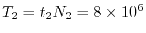
Since two different types of numerical algorithms for SBT are available
in LIBERI, two different types of SBT-mesh are provided, namely the
logarithmic mesh and linearly-spaced mesh.
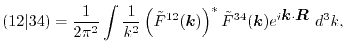
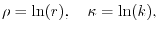
The schematic illustration of the meshes is shown in Fig. 1.
Figure 1:
Schematic illustration of the two kinds of radial meshes used in LIBERI.
|
The logarithmic mesh covers from  to
to
 with
with  points where the interval between two adjacent points becomes
exponentially wider as
points where the interval between two adjacent points becomes
exponentially wider as  increases.
Most of the points are thus located in the vicinity of .
This is suitable to describe atomic orbital wave functions in real
space since the detailed structure near nuclei is well described.
While, in reciprocal space, it is not so suitable because the important
information is contained in the partial waves at large wave numbers.
In fact, the Gaussian-type damping term described in
Eq. (18) screens out the contributions from the small wave
numbers region.
The linearly-spaced mesh covers from 0 to
with N
points which are separated by a uniform interval
increases.
Most of the points are thus located in the vicinity of .
This is suitable to describe atomic orbital wave functions in real
space since the detailed structure near nuclei is well described.
While, in reciprocal space, it is not so suitable because the important
information is contained in the partial waves at large wave numbers.
In fact, the Gaussian-type damping term described in
Eq. (18) screens out the contributions from the small wave
numbers region.
The linearly-spaced mesh covers from 0 to
with N
points which are separated by a uniform interval
 .
For the convenience in performing FFT, the mesh points are shifted by a
half of the interval.
.
For the convenience in performing FFT, the mesh points are shifted by a
half of the interval.
In LIBERI, two different kinds of numerical methods for SBT are
available.
One is developed by Siegman [12] and
Talman [13], which is one of the most established method
for the numerical SBT.
In the method, a SBT is evaluated through two consecutive Fourier
transforms, by employing a logarithmic radial mesh.
The other method for numerical SBT has recently been developed by the
authors [14] which shows performance comparable to or
even better in some specific cases than the Siegman-Talman method.
This method uses a linearly spaced radial mesh.
For convenience sake, the methods are called as log-FSBT and
linear-FSBT, respectively, where FSBT stands for fast
spherical Bessel transform.
The log-FSBT is faster for a single transform, while the linear-FSBT
is faster for a series of transforms.
As the overall performance, the calculations of the overlap functions
with the liner-FSBT method is faster (by only a few percent, though)
than the calculations with the log-FSBT method.
Therefore, the linear-FSBT is used in LIBERI as the default setting.
The radial coordinate variables and  are replaced by their
logarithms,
are replaced by their
logarithms,
 |
(21) |
so that a SBT becomes a convolution-type integral as follows:
where  is an integer lying between 0 and
  and
and
 is defined as
 |
(23) |
The function
can be expressed
analytically [13].
The integer determines the accuracy of this conversion via the
factor
 in Eq. (22).
High accuracy can be achieved with
in Eq. (22).
High accuracy can be achieved with  for
for
 and
and
 for
for
 [13].
In out implementation, is set to be 0 unless explicitly specified.
The Fourier transforms in Eq. (22) are performed
numerically by the fast Fourier transform (FFT) algorithm.
The computation effort of the log-FSBT method, therefore,
scales as
[13].
In out implementation, is set to be 0 unless explicitly specified.
The Fourier transforms in Eq. (22) are performed
numerically by the fast Fourier transform (FFT) algorithm.
The computation effort of the log-FSBT method, therefore,
scales as
 .
.
The authors have recently developed a new method for numerical
SBT [14] aiming to overcome the restriction of the
shape of the radial mesh.
The starting point of the method is the integral representation of the
spherical Bessel function,
 |
(24) |
where  is the Legendre polynomial.
By substituting Eq. (24) into the SBT, the following
expression is obtained:
is the Legendre polynomial.
By substituting Eq. (24) into the SBT, the following
expression is obtained:
where
 is the Fourier cosine/sine transform of
,
is the Fourier cosine/sine transform of
,
By expanding the Legendre polynomial explicitly, Eq. (25)
becomes
where  is a double factorial and
  is defined as
The integration in Eq. (28) is carried out by piecewise
integration where each piece is evaluated by using a cubic polynomial
interpolation.
Since the integrand does not depend on , the values of for
all points are obtained in an efficient recursive
manner [14].
The derivatives of of
 with respect to
  is also required
for the polynomial interpolation, which are easily derived as follows:
is also required
for the polynomial interpolation, which are easily derived as follows:
Note that the order of appearing in Eq. (25) is
always of the same parity as the order of transform , which means
that either cosine of sine transform in Eqs. (26) and
(29) is required to be evaluated.
Therefore, the required number of the Fourier transforms in the
linear-FSBT method is two, which is equivalent to the number required in
the log-FSBT method.
In addition to the FFT operations, the linear-FSBT method requires the
integrations described in Eq. (28).
Nevertheless, the total computation time of the linear-FSBT in actual
calculations is in the same order as that of the log-FSBT method.
Table 1:
Computation time in msec for a set of transforms by
the log-FSBT and linear-FSBT methods, where a function is
transformed with each different order from 0 to 14.
The number of sampling points is 2048.
In result A, the redundant computations are skipped within a
serial transform. Note that the skipping is applied to the
log-FSBT method as well as the linear-FSBT method.
In result B, every transform is performed one by one, without
using the skipping.
The computation was perform on a PC with Intel Core i7
processors @ 2.67 GHz.
| (msec) |
log-FSBT |
linear-FSBT |
| A |
6.8 |
3.4 |
| B |
9.6 |
22.8 |
|
The most significant advantage of the linear-FSBT method is gained when
an input function is transformed for several different orders, which
happens, for example, in the evaluation of
 in Eq. (7).
Since appearing in Eq. (26) does not depend on
the order of transform (nor equivalently on ), the most time
consuming part (the Fourier transforms and the integration in
Eq. (28)) can be skipped after the first operation.
In Table 1, results of test calculations where a function
is transformed for a series of orders up to 14 are shown.
The linear-FSBT method is twice faster than the log-FSBT method when
redundant computations are skipped.
in Eq. (7).
Since appearing in Eq. (26) does not depend on
the order of transform (nor equivalently on ), the most time
consuming part (the Fourier transforms and the integration in
Eq. (28)) can be skipped after the first operation.
In Table 1, results of test calculations where a function
is transformed for a series of orders up to 14 are shown.
The linear-FSBT method is twice faster than the log-FSBT method when
redundant computations are skipped.
Expansion Centers
The convergence speed of -summation in Eq. (15) depends
on the choice of the positions of and .
In LIBERI, in order to make the equations of the derivative simpler,
every center is assumed to be located on a line segment between the
centers of two basis functions.
For example, the center of the overlap functions between the basis
functions
and
located at
and , respectively, is given as
 |
 |
(30) |
where  and
and  are parameters which are functionals
of the basis functions.
The simplest choice is the middle-point (
are parameters which are functionals
of the basis functions.
The simplest choice is the middle-point (
 ).
A more reasonable choice is to make and proportional
to the inverse of
).
A more reasonable choice is to make and proportional
to the inverse of
 .
Talman [15] has investigated the convergence
speed of an exchange integral defined by
.
Talman [15] has investigated the convergence
speed of an exchange integral defined by
where  and
and  are STOs with different orbital
parameters and
are STOs with different orbital
parameters and
 , showing that the convergence
becomes faster with the expansion centers at the
, showing that the convergence
becomes faster with the expansion centers at the
 -averaged points than with those at the
middle-points.
-averaged points than with those at the
middle-points.
Another choice is to make and proportional to
the
 .
Although
characterizes the averaged
distribution of the radial function, it does not distinguish
the anisotropic shapes between, for example,
.
Although
characterizes the averaged
distribution of the radial function, it does not distinguish
the anisotropic shapes between, for example,  and
and  orbitals.
By introducing
orbitals.
By introducing
 , the spatial anisotropy
of the basis function is effectively taken into account.
We have calculated the exchange integral where and
are PAO wave functions with different spatial extents,
namely the
, the spatial anisotropy
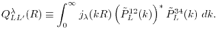
of the basis function is effectively taken into account.
We have calculated the exchange integral where and
are PAO wave functions with different spatial extents,
namely the  orbital of H atom and
  orbital of Na atom.
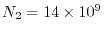
The radial parts of and are plotted in
Fig. 2,
The convergence behavior of the exchange integral with different
expansion centers is shown in Table 2 for
orbital of Na atom.
The radial parts of and are plotted in
Fig. 2,
The convergence behavior of the exchange integral with different
expansion centers is shown in Table 2 for
 and
and  , where the labels C1, C2, and C3 indicate the
choice of the centers at the middle-points,
the
-averaged points,
and the
-averaged
points, respectively.
For case, the exchange integral converges much faster with
the centers at C2 and C3, than with the centers at C1.
We have also checked the convergence speed of the exchange integral for
different values of
, where the labels C1, C2, and C3 indicate the
choice of the centers at the middle-points,
the
-averaged points,
and the
-averaged
points, respectively.
For case, the exchange integral converges much faster with
the centers at C2 and C3, than with the centers at C1.
We have also checked the convergence speed of the exchange integral for
different values of  .
As summarized in Table 3, the convergence speed with
the centers at C2 and C3 is almost the same and generally faster than C1.
Since the speed with C3 is slightly faster than that with C2,
LIBERI employs the
-averaged
points as the default choice of the expansion centers.
.
As summarized in Table 3, the convergence speed with
the centers at C2 and C3 is almost the same and generally faster than C1.
Since the speed with C3 is slightly faster than that with C2,
LIBERI employs the
-averaged
points as the default choice of the expansion centers.
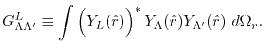
Figure 2:
PAO wave functions for orbital of H atom (solid line) and
orbital of Na atom (dashed line) where the confinement radii are
 a.u. and
  a.u., respectively.
|
How to compile
The source files of LIBERI is distributed in a gzipped tar archive
format.
A typical way to extract the source files is
tar vxf liberi-*.tar.gz
or equivalently
gunzip < liberi-*.tar.gz | tar vx
Since LIBERI is a set of C subroutines, the users can easily
combine LIBERI with their own C program codes.
In order to avoid name conflicts, each source file is given
a name starting with prefix ERI_, and every variable
and function with external linkage has a name starting with
prefix eri_.
As another option, the users can compile LIBERI as an archive library
and link it with their program afterwards.
A simple makefile is included in the distribution package.
The makefile should be edited, so that some environment variables are
correctly defined.
In a correct makefile,
- CC specifies the C compiler,
- OPT holds the optimization options for the compiler, and
- FFTW_INCLUDE_DIR points the directory where
fftw3.h is located.
Then, the archive library of LIBERI can be compiled by typing
make
If the compilation is succeeded, the archive library file liberi.a
is created.
The users can combine LIBERI with their own program by including the
header file eri.h and linking it with liberi.a.
LIBERI uses two other external libraries, BLAS [16] and
FFTW [17].
The users have to link these libraries with their own program which
uses LIBERI.
How to use
Before any operation of LIBERI can be performed, LIBERI must be
initialized by calling ERI_Init which allocates workspace memory,
defines the radial grids, calculates target-independent components such
as the Gaunt coefficients, and returns a pointer to an object that
contains all the relevant information.
To release the workspace memory, the users should simply call
ERI_Free passing the pointer returned by ERI_Init.
In general, the evaluation of ERI is performed by calling the low-level
functions of LIBERI one-by-one, as follows:
ERI_Transform_Orbital
performs SBT of orbital functions,
ERI_LL_Gamma
calculates
according to
Eq. (7),
ERI_LL_Alpha
calculates
 according to
Eq. (6),
ERI_LL_Overlap
calculates the overlap function
according to
Eq. (6),
ERI_LL_Overlap
calculates the overlap function
 according to
Eq. (11),
ERI_Transform_Overlap
performs SBT of the overlap functions,
ERI_GL_Interpolation
changes the radial grid from SBT-mesh to GL-mesh,
and ERI_Integral_GL
performs the integration in Eq. (16) and summation
in Eq. (15).
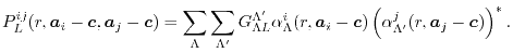
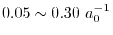
The sequence of the calculation is schematically shown in
Fig. 3 where data is indicated by the square boxes and
the low-level functions by the rounded boxes.
The arrays to store the intermediate components such -functions
and the overlap functions have to be allocated by the users.
All the arrays are of double type and the
required byte size can be obtained by calling ERI_Size_of_*
functions.
For example, an array for -functions is safely allocated
by the following code:
according to
Eq. (11),
ERI_Transform_Overlap
performs SBT of the overlap functions,
ERI_GL_Interpolation
changes the radial grid from SBT-mesh to GL-mesh,
and ERI_Integral_GL
performs the integration in Eq. (16) and summation
in Eq. (15).
The sequence of the calculation is schematically shown in
Fig. 3 where data is indicated by the square boxes and
the low-level functions by the rounded boxes.
The arrays to store the intermediate components such -functions
and the overlap functions have to be allocated by the users.
All the arrays are of double type and the
required byte size can be obtained by calling ERI_Size_of_*
functions.
For example, an array for -functions is safely allocated
by the following code:
double *alpha;
alpha = (double*)malloc( ERI_Size_of_Alpha(eri) );
where eri is the pointer returned by ERI_Init.
For the users who do not wish to be bothered with memory management,
LIBERI provides several black box functions which perform necessary
calculations by calling the low-level functions internally.
The schematic structure of the black box functions are illustrated
in Fig. 3 by the rounded boxes with dashed lines.
Figure 3:
Illustration of the calculation process of LIBERI.
The low-level routines are indicated by the rounded boxes
with solid lines.
The input and output data of the routines are indicated by the square
boxes with the arrows.
The high-level (black box) routines are indicated by the
rounded boxes with dashed lines.
The shaded areas show two distinct part of the
process.
In the procedure 1, the SBT-mesh with the parameters
 and
and
 are used, while in the procedure 2, the GL-mesh with
the
parameters
are used, while in the procedure 2, the GL-mesh with
the
parameters
 and
and
 are used.
|
One quick example how to use LIBERI is given in the following:
ERI_t *eri;
ERI_Orbital_t *p1, *p2, *p3, p4;
ERI_Info_t *info;
double screen, I4[2], dI4[2];
int lmax, lmax_gl, ngrid, ngl;
...
eri = ERI_Init(lmax, lmax_gl, ngrid, ngl, info);
ERI_Integral(eri, I4, dI4, p1, p2, p3, p4, screen);
ERI_Free(eri);
The arguments for ERI_Init are:
lmax is the maximum value of angular momentum
,
lmax_gl the cut-off of the summation
,
ngrid the number of SBT-mesh points,
ngl the number of the GL-mesh points,
and
info the additional parameters for tuning the performance and for
debugging.
If info is NULL, the default settings are used.
After LIBERI is initialized, the integral are calculated by calling
ERI_Integral.
The information of basis functions should be stored in
ERI_Orbital_t object which is defined as:
typedef struct {
  double       *fr;
  double       *xr;
  unsigned int  ngrid;
  int           l;
  int           m;
  double        c[3];
} ERI_Orbital_t;
where fr is a pointer to an array for the radial wave function
, xr a pointer to an array for the radial mesh in atomic
units, ngrid the number of items of fr and xr,
l the orbital angular momentum, m the spin angular
momentum, and c the position of the basis function in the
Cartesian coordinate in atomic units.
For the calculation of the integral with the unscreened (bare)
Coulomb interaction, screen should be ERI_NOSCREEN, while,
for the calculation of the integral with the screened
Coulomb interaction, screen should be the screening parameter
in unit of  .
The calculated integral is stored in I4 and the derivatives
in dI4.
If the derivatives are not needed, dI4 can be NULL and
the calculations for the derivatives are skipped.
.
The calculated integral is stored in I4 and the derivatives
in dI4.
If the derivatives are not needed, dI4 can be NULL and
the calculations for the derivatives are skipped.
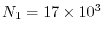
Computation time
On a PC cluster with Intel Xeon processor @ 2.83 GHz, the averaged time
for calculating one integral is  sec where the procedure 1
(see Fig. 3) spends
sec where the procedure 1
(see Fig. 3) spends  msec and the procedure 2
spends
msec and the procedure 2
spends
 msec, where
 ,
,
 ,
,
 ,
and
,
and
 .
As a quick estimation, let us consider a bulk GaAs crystal in the
zincblende structure with the lattice constant
.
As a quick estimation, let us consider a bulk GaAs crystal in the
zincblende structure with the lattice constant
 .
There are two atoms in the unit cell and 13 PAO basis functions are
assigned to each atom.
The truncation of the PAO functions is
.
There are two atoms in the unit cell and 13 PAO basis functions are
assigned to each atom.
The truncation of the PAO functions is
 and the screening parameter is chosen to be
 which corresponds to the cut-off length
 for the Coulomb interaction at an accuracy of
Hartree [11].
In this condition, the number of pairs of basis functions is
for the Coulomb interaction at an accuracy of
Hartree [11].
In this condition, the number of pairs of basis functions is
 and the number of quartet of basis functions is
 .
The estimated time for the procedure 1 and 2 is
.
The estimated time for the procedure 1 and 2 is
 sec and
 sec, respectively.
Therefore, the total time required for a calculation of bulk GaAs
is determined almost solely by
sec, respectively.
Therefore, the total time required for a calculation of bulk GaAs
is determined almost solely by  .
The ERI given in Eq. (19) has a symmetry in permutation of
the basis functions as follows:
.
The ERI given in Eq. (19) has a symmetry in permutation of
the basis functions as follows:
The estimated time is
 days without using parallele
computation nor skipping computations when the overlap function
days without using parallele
computation nor skipping computations when the overlap function
 is small enough.
As shown above,
is small enough.
As shown above,  is very much smaller than
  , so that the
computation cost for the procedure 1 is negligible even though
, so that the
computation cost for the procedure 1 is negligible even though  is
significantly larger then
is
significantly larger then  .
This is due to the strict locality of the PAO basis functions.
The performance of our code is, thus, characterized by and is
comparable to other established programs.
For example, in one of the fastest code based on the Gaussian-expansion
method [18], averaged computation cost for a single three-
or four-center integral with STO basis sets is 0.5 - 1.5 msec where
the number of GTOs for a STO is 12 - 15.
.
This is due to the strict locality of the PAO basis functions.
The performance of our code is, thus, characterized by and is
comparable to other established programs.
For example, in one of the fastest code based on the Gaussian-expansion
method [18], averaged computation cost for a single three-
or four-center integral with STO basis sets is 0.5 - 1.5 msec where
the number of GTOs for a STO is 12 - 15.
Summary
In conclusion, we present a new library called LIBERI for computing the
multicenter electron repulsion integrals for numerically defined basis
functions based on successive reduction of integral dimension.
It is written in standard C in an easy and well structured coding style.
All necessary low-level functions which correspond to the equations
described in the present paper as well as a user-friendly black box
functions are provided.
We believe that LIBERI is easy to be combined to electronic structure
calculation codes which employ localized basis functions.
Development of an interface code for implementation of the hybrid
functional methods to OpenMX [8,19,20] is in
progress.
Acknowledgments
This work was partly supported by CREST-JST and the Next Generation
Super Computing Project, Nanoscience Program, MEXT, Japan.
- 1
-
S. F. Boys, Electronic wave functions I. A general method of calculation for
the stationary states of any molecular system A200 (1950) 542.
- 2
-
I. Shavitt, M. Karplus, Gaussian-Transform Method for Molecular Integrals. I.
Formulation for Energy Integrals, J. Chem. Phys. 43 (1965) 398.
- 3
-
H. Taketa, S. Huzinaga, K. O-ohata, Gaussian-Expansion Methods for Molecular
Integrals, J. Phys. Soc. Jpn 21 (1966) 2313.
- 4
-
P. M. W. Gill, J. A. Pople, Int. J. Quantum Chem. 40 (1991) 753.
- 5
-
K. Ishida, ACE Algorithm for the Rapid Evaluation of the Electron-Repulsion
Integral over Gaussian-Type Orbials, Int. J. Quantum Chem. 59 (1996) 209.
- 6
-
J. D. Talman, Numerical Methods for Multicenter Integrals for Numerically
Defined Basis Functions Applied in Molecular Calculations, Int. J. Quantum
Chem. 93 (2003) 72.
- 7
-
M. Toyoda, T. Ozaki, Numerical evaluation of electron repulsion integrals for
pseudoatomic orbitals and their derivatives, J. Chem. Phys. 130 (2009)
124114.
- 8
-
T. Ozaki, H. Kino, Numerical atomic basis orbitals from H to Kr, Phys. Rev. B
69 (2004) 195113.
- 9
-
P.-O. Löwdin, Quantum Theory of Cohesive Properties of Solids, Adv. Phys. 5
(1056) 1.
- 10
-
D. Pines, Elementary Excitations in Solids, Perseus Books, Reading, MA, 1999.
- 11
-
J. Heyd, G. E. Scuseria, M. Ernzerhof, Hybrid functionals based on a screened
Coulomb potential, J. Chem. Phys. 118 (2003) 8207.
- 12
-
A. E. Siegman, Quasi fast Hankel transform, Opt. Lett. 1 (1977) 13.
- 13
-
J. D. Talman, Numerical Fourier and Bessel Transforms in Logarithmic Variables,
J. Comput. Phys. 29 (1978) 35.
- 14
-
M. Toyoda, T. Ozaki, Fast spherical Bessel transform via fast Fourier transform
and recurrence formula, submitted to Computer Physics Communictions (2009).
- 15
-
J. D. Talman, Multipole Expansions for Numerical Orbital Products, Int. J.
Quantum Chem. 107 (2007) 1578.
- 16
-
BLAS Home Page,
http://www.netlib.org/blas/.
- 17
-
M. Frigo, S. G. Johnson, FFTW Home Page,
http://www.fftw.org/.
- 18
-
J. F. Rico, R. López, I. Ema, G. Ramírez, Efficiency of the Algorithms for
the Calculation of Slater Molecular Integrals in Polyatomic Molecules, J.
Comput. Chem. 25 (2004) 1987.
- 19
-
T. Ozaki, H. Kino, Efficient Projector Expansion for the Ab Initio LCAO Method,
Phys. Rev. B 72 (2005) 045121.
- 20
-
T. Ozaki, OpenMX website,
http://www.openmx-square.org.
LIBERI: Library for Numerical Evaluation of Electron-Repulsion Integrals
This document was generated using the
LaTeX2HTML translator Version 2002-2-1 (1.71)
Copyright © 1993, 1994, 1995, 1996,
Nikos Drakos,
Computer Based Learning Unit, University of Leeds.
Copyright © 1997, 1998, 1999,
Ross Moore,
Mathematics Department, Macquarie University, Sydney.
TOYODA Masayuki
2010-07-01
![\includegraphics[width=0.5\textwidth]{fig2.eps}](fig2.png)
![\includegraphics[width=0.9\textwidth]{fig3.eps}](fig3.png)


![\includegraphics[width=0.6\textwidth]{fig1.eps}](fig1.png)