Accurate finite element method for atomic calculations based on density functional theory and Hartree-Fock method

Taisuke Ozaki (JAIST) and Masayuki Toyoda (JAIST)

Copyright 2011 Elsevier B.V. This article is provided by the author for the reader's personal use only. Any other use requires prior permission of the author and Elsevier B.V. NOTICE: This is the author's version of a work accepted for publication by Elsevier. Changes resulting from the publishing process, including peer review, editing, corrections, structural formatting and other quality control mechanisms, may not be reflected in this document. Changes may have been made to this work since it was submitted for publication. A definitive version is subsequently published in Computer Physics Communications 182, 1245-1252 (2011), DOI:10.1016/j.cpc.2011.02.010 and may be found at here.

Abstract:

An accurate finite element method is developed for atomic calculations based on density functional theory (DFT) within local density approximation (LDA) and Hartree-Fock (HF) method. The radial wave functions are expanded by cubic Hermite spline functions on a uniform mesh for $x=\sqrt{r}$, and all the associated integrals are analytically evaluated in conjunction with fitting procedures of the hartree and the exchange-correlation potentials to the same cubic Hermite spline functions using a set of recurrence formulas. The total energy of atoms systematically converges from above, and the error algebraically decays as the mesh spacing decreases. When the mesh spacing $d$ is taken to be $0.025/\sqrt {Z}$ bohr$^{1/2}$, the total energy for an atom of atomic number $Z$ can be calculated within error of $10^{-7}$ hartree for both the LDA and HF methods. The equal applicability of the method to DFT and the HF method with a similar degree of high accuracy enables the method to be a reliable platform for development of new functionals in DFT such as hybrid functionals.

INTRODUCTION

The electronic structure calculation of atoms[1,2] is one of most fundamental bases in not only understanding electronic structures of molecules and solids, but also developing efficient and accurate electronic structure methods. For the latter case, it is indispensable to distinguish the intrinsic error produced by the theoretical framework itself from that caused by the other numerical problems such as incompleteness of basis set and inaccurate numerical integration,[3] which will be referred to as non-intrinsic error hereafter. If the non-intrinsic error is extremely small, the validation of electronic structure methods can be very precisely performed, which may highlight strength and weakness of each method without suffering from any appreciable numerical error. By the recent advance of the electronic structure methods, requirement for the intrinsic error has been approaching chemical accuracy (1mHartree).[4,5,6] One can imagine that the requirement for the intrinsic error should be smaller than the chemical accuracy for further development of accurate electronic structure methods. A potential approach which can minimize the non-intrinsic error is a finite element (FE) method in which wave functions are expressed by a linear combination of piecewise polynomial functions. [7,8,10,9,11,12,13,14,15,16] Since the approach based on the FE method can be regarded as a traditional basis set method, once a highly accurate FE method is established, it is apparent for the FE method to be widely used as a platform for development of new functionals in density functional theory (DFT)[17,18] and post Hartre-Fock (HF) methods. The equal applicability of the method to DFT and the HF method with a similar degree of high accuracy is also highly important because hybrid methods, in which DFT and wave function theories such as the HF method are unified in a single framework, have recently attracted much attention.[6,19,20,21,22,23] Although a wide variety of FE methods have been already developed for atomic calculations so far,[7,8,10,9,11,12] the equal applicability of the method to DFs and wave function theories has not been clearly established. In DFT calculations numerical integrations have to be essentially employed due to non-analytic nature of exchange-correlation functionals, while two electron repulsion integrals can be calculated analytically in wave function theories such as the HF method. The difference in evaluating matrix elements for exchange-correlation potentials limits the equal applicability of each method to DFs and wave function theories with a similar degree of high accuracy. In this paper, in order to establish a basis for development of electronic structure methods which may consist of a DF and a wave function theory, we present an accurate finite element method for atomic calculations based on not only DFT, but also the HF method. To address the equal applicability of the method to DFs and wave function theories, we use one of the simplest piecewise polynomial functions, i.e., cubic Hermite spline functions, as basis functions, and show that the use of the cubic Hermite spline functions allows one to analytically evaluate all of integrals involved in conjunction with fitting procedures of the hartree and the exchange-correlation potentials to the same cubic Hermite spline functions. As a result of the analytic evaluation of matrix elements, it is found that the non-intrinsic error in the DFT and HF calculations can be systematically reduced by only decreasing the mesh spacing, and that eventually the FE method can provide numerically exact solutions within machine precision for all the atoms (Z=1-103) in the periodic table. This paper is organized as follows: In Sec. II the theoretical framework of the FE method using the cubic Hermite spline functions is presented for DFT within local density approximation (LDA) and the HF method. In Sec. III numerical accuracy of the FE method is demonstrated by the total energy energy calculations of all the atoms (Z=1-103) in the periodic table. In Sec. IV we summarize the FE method, and discuss a future possible application of the method in development of a new functional in DFT. Throughout the paper, we use atomic units, where $\hbar=e^2=m_{\rm e}=1$.

FINITE ELEMENT METHOD

Local density functional

Let us start to write the one particle wave function $\psi_{nlm}$ as

$$\psi_{nlm}({\bf r}) = Y_{lm}(\hat{{\bf r}})R_{nl}(r),$$ (1)

where $Y_{lm}$ and $R_{nl}$ are a spherical harmonic and a radial wave function, respectively. By introducing change of variables $r = x^2$,[24] which allows us to eliminate the cusp of wave functions at the origin in $x$-coordinate, and assuming a spherical potential $V(x)$, the radial Schrödinger equation is given by

$$\hat{H}R_{nl}(x) = \varepsilon_{nl} R_{nl}(x)$$ (2)

with

$$\hat{H} = \hat{T_0}+\hat{T_1}+ V(x),$$ (3)

where the operators $\hat{T_0}$ and $\hat{T_1}$ are defined by

$$\hat{T_0} = -\frac{1}{8x^2}\frac{d^2}{dx^2} -\frac{3}{8x^3}\frac{d}{dx},$$ (4)

$$\hat{T_1} = \frac{l(l+1)}{2x^4},$$ (5)

and the potential $V(x)$ is the sum of three contributions:

$$V(x) = \frac{-Z}{x^2} + V_{\rm H}(x) + V_{\rm xc}(x).$$ (6)

The first term is the attractive potential of the nucleus with atomic number $Z$, and the second and third are the hartree and exchange correlation potentials, respectively. Although we restrict ourselves to the spherical potential in the paper, the FE method we discuss may be generalized to the non-spherical case by combining with the Slater method.[2] We now expand the radial function $R(x)$ using cubic Hermite spline functions $S$ as basis functions[28], which are placed on a regular mesh with spacing $d$ in $x$-coordinate, as follows:

$$R_{nl}(x) = \sum_{i=0}^{N-1}\sum_{k=0}^{1} c^{(nl)}_{ik}S_{k}^{(i)}(\frac{x-x_{i}}{d}),$$ (7)

where the spacing is determined by $d\equiv x_{\rm max}/(N-1)$, and $S_0$ and $S_1$, shown in Fig. 1(a), are defined by

$$S_{0}(x) = \left\{ \begin{array}{rl} 1 - 3x^2 + 2x^3, &\quad {\rm0\leq x\leq... ...x), &\quad {\rm -1\leq x< 0}\\ 0, &\quad {\rm otherwise}\\ \end{array}\right.$$ (8)

$$S_1(x) = \left\{ \begin{array}{rl} x - 2x^2 + x^3, &\quad {\rm0\leq x\leq ... ...x), &\quad {\rm -1\leq x< 0}\\ 0, &\quad {\rm otherwise}\\ \end{array}\right.$$ (9)

The spline function $S_0$ satisfies a set of conditions that $S_{0}(0)=1$, $S_{0}'(0)=0$, and $S_{0}(\pm 1)=S_{0}'(\pm 1)=0$, while $S_1$ satisfies $S_{1}(0)=0$, $S_{1}'(0)=1$, and $S_{1}(\pm 1)=S_{1}'(\pm 1)=0$. The superscript $(i)$ for $S_{k}^{(i)}$ in Eq. (7) means that the origin of $S_{k}$ is shifted to $x_i$, where $x_i$ is given by $id$.

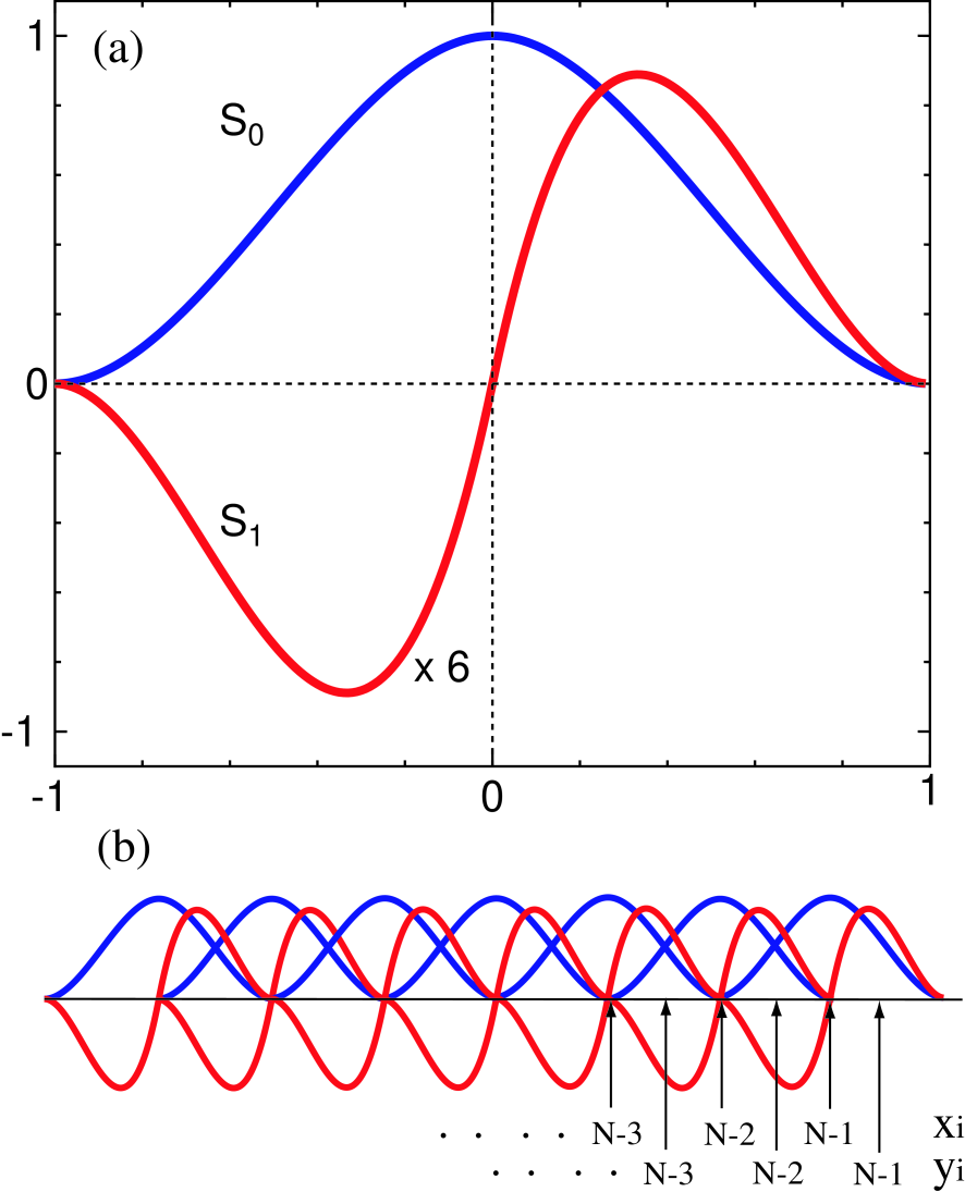
Figure 1: (Color online) (a) Cubic Hermite spline functions $S_0$ and $S_1$ defined by Eqs. (8) and (9). (b) Two sorts of regular meshes $\{x_i\}$ and $\{y_i\}$ in $x$-coordinate, which are used for fitting of the hartree and exchange-correlation potentials.

The accuracy in description of $R$ can be systematically controlled by increasing $N$ as shown later. Employing Eq. (7) for Eq. (2) readily gives the following generalized eigenvalue problem:

$$Hc = \varepsilon Sc,$$ (10)

where $H$ and $S$ are the hamiltonian and overlap matrices, respectively, and these matrices becomes septuple diagonal in LDA, since basis functions $S^{(i)}$ interact with basis functions $S^{(i\pm 1)}$ in the nearest neighbor sites $i\pm 1$. All the matrix elements, except for that of the exchange-correlation potential such as LDA,[25,26] can be analytically evaluated. For example, all the non-zero matrix elements for the operator $\hat{T_{0}}$ are found to be

off-site elements

$$%% off-site \langle S_0^{(i)} \vert \hat{T_{0}} \vert S_0^{(i+1)} \rangle = \frac{-3d^2}{280}(5+24i+42i^2+28i^3),$$ (11)

$$\langle S_0^{(i)} \vert \hat{T_{0}} \vert S_1^{(i+1)} \rangle = \frac{d^2}{560}(-5-12i+14i^3),$$ (12)

$$\langle S_1^{(i)} \vert \hat{T_{0}} \vert S_0^{(i+1)} \rangle = \frac{-d^2}{560}(7+30i+42i^2+14i^3),$$ (13)

$$\langle S_1^{(i)} \vert \hat{T_{0}} \vert S_1^{(i+1)} \rangle = \frac{-d^2}{3360}(11+36i+42i^2+28i^3),$$ (14)

on-site elements for $i\neq 0$

$$%% on-site \langle S_0^{(i)} \vert \hat{T_{0}} \vert S_0^{(i)} \rangle = \frac{3d^2}{35}(6i+7i^3),$$ (15)

$$\langle S_0^{(i)} \vert \hat{T_{0}} \vert S_1^{(i)} \rangle = \langle S_1^{(i)} \vert \hat{T_{0}} \vert S_0^{(i)} \rangle = \frac{d^2}{40}(1+6i^2),$$ (16)

$$\langle S_1^{(i)} \vert \hat{T_{0}} \vert S_1^{(i)} \rangle = \frac{d^2}{105}(3i+7i^3),$$ (17)

on-site elements for $i=0$

$$%% on-site, in case of i=0 \langle S_0^{(0)} \vert \hat{T_{0}} \vert S_0^{(0)} \rangle = \frac{15d^2}{208},$$ (18)

$$\langle S_0^{(0)} \vert \hat{T_{0}} \vert S_1^{(0)} \rangle = \langle S_1^{(0)} \vert \hat{T_{0}} \vert S_0^{(0)} \rangle = \frac{d^2}{80},$$ (19)

$$\langle S_1^{(0)} \vert \hat{T_{0}} \vert S_1^{(0)} \rangle = \frac{11d^2}{3360}.$$ (20)

It turns out that the matrix elements depend on the site $i$ as a result that the extent of region spanned by the basis function in $r$-coordinate varies depending on the site $i$. Also it is noted that four on-site matrix elements at $i=0$ have to be calculated by taking account of a fact that the basis functions $S^{(0)}$ span only the region ranging from $0$ to $d$ in $x$-coordinate, resulting in Eqs. (18)-(20). As well as $\hat{T_{0}}$, the matrix elements for $\hat{T_{1}}$, $-Z/x^2$, and $V_{\rm H}(x)$ and the overlap matrix elements can be analytically evaluated, and all the analytic formulas and MATHEMATICA codes for generating them are provided in Secs. S-1-12 of the supplemental material. Although the matrix elements for $V_{\rm H}$ can be analytically evaluated as shown in the section of HF method, for the LDA calculation we present an alternative numerical method which is much faster than the analytic counterpart, while keeping numerical accuracy. Thus, one may see that in LDA the remaining matrix elements which are numerically evaluated are only those for the hartree and exchange-correlation potentials in the FE method.

Here we show that even the matrix elements for the hartree and exchange-correlation potentials can be very accurately evaluated by utilizing the same cubic spline functions in the FE method. Let us introduce two sorts of regular meshes with spacing $d$ in $x$-coordinate, that is, one is $x_i$ as defined before and the other $y_i\equiv d(i+\frac{1}{2})$, as shown in Fig. 1(b). We evaluate the charge density $n$ on the two regular meshes, where, by recalling that the basis functions are strictly localized in real space, one can compute the charge density $n$ by considering only contributions of the neighboring sites at each mesh point, and fit the charge density on the meshes to the following function:

$$n(x) = \sum_{i=0}^{N-1} \left( a_{i}S_{0}^{(i)}(\frac{x-x_{i}}{d}) +b_{i}S_{1}^{(i)}(\frac{x-x_{i}}{d}) \right),$$ (21)

where $a_{i}$ and $b_{i}$ are uniquely determined by a set of recurrence formulas:

$$a_{i} = n(x_i),$$ (22)

$$b_{i} = \left\{ \begin{array}{rl} 8n(y_{i}) - 4a_{i}, &\quad {\rm i=N-1}\... ...n(y_{i})-4a_{i}-4a_{i+1}+b_{i+1}, &\quad {\rm i\neq N-1},\\ \end{array}\right.$$

The recurrence formulas are derived by noting that only $S_{0}^{(i)}$ is non-zero at $x_i$ as shown in Fig. 1(b) and that $b_i$ is only the unknown parameter if we start to fit $\{V_{\rm xc}(y_i)\}$ to the function Eq. (21) from $y_{N-1}$, which results in that Eq. (23) has to be recursively solved starting from $i=N-1$. Once $n$ is expanded in terms of the Hermite spline functions, by considering the spherical charge density distribution, we can analytically evaluate the hartree potential as

$$V_{\rm H}(x_i) = \frac{8\pi}{x_i^2}\int_{0}^{x_i}n(x')x'^5dx' + 8\pi\int_{x_i}^{\infty}n(x')x'^3dx',$$

where the integrals are analytically evaluated due to the integrands by simple polynomial functions. As well, $\{V_{\rm H}(y_i)\}$ on the other mesh $y_i$ are calculated in the same way as for $\{V_{\rm H}(x_i)\}$. The explicit formulas of the integrals can be found in Secs. S-13 and 14 of the supplemental material. Using the similar way to the expansion of charge density, the set of $\{V_{\rm H}(x_i)\}$ and $\{V_{\rm H}(y_i)\}$ can be fitted to

$$V_{\rm H}(x) = \sum_{i=0}^{N-1} \left( A_{i}S_{0}^{(i)}(\frac{x-x_{i}}{d}) +B_{i}S_{1}^{(i)}(\frac{x-x_{i}}{d}) \right),$$

where the coefficients $A_{i}$ and $B_{i}$ are uniquely determined by the similar recurrence formulas to Eqs. (22) and (23). Once $\{V_{\rm H}(x_i)\}$ and $\{V_{\rm H}(y_i)\}$ are fitted to Eq. (25), the calculation of matrix elements for $V_{\rm H}(x)$ is straightforward as follows:

$${ \langle S_{k}^{(i)} \vert V_{\rm H} \vert S_{k'}^{(j)} \rangle = }$$

$$\sum_{p=0}^{N-1} \left( A_{i} \langle S_{k}^{(i)} \vert S_{0}^{(p... ...B_{i} \langle S_{k}^{(i)} \vert S_{1}^{(p)} \vert S_{k'}^{(j)} \rangle \right).$$ (23)

The integrals involved survive only if $p=i-1, i$, or $i+1$ for $i=j$, and $p=i$ or $j$ for $\vert i-j\vert=1$, and there are 24 and 16 non-zero elements for the former and the latter, respectively, which can be easily evaluated in analytic formulas. The other combinations give always zero elements due to the strictly localized spline functions. All the analytic formulas and MATHEMATICA codes for generating them are provided in Secs. S-15-21 of the supplemental material. The matrix elements for the exchange-correlation potential can be calculated by just replacing $V_{\rm H}$ with $V_{\rm xc}$ in Eqs. (25) and (26) after $\{V_{\rm xc}(x_i)\}$ and $\{V_{\rm xc}(y_i)\}$ are calculated by LDA. Thus, from the above derivation we see that all the matrix elements required in the FE method within LDA are evaluated without introducing numerical integration which can be a serious source of numerical error. It is also pointed out that the extension of the method to generalized gradient approximation (GGA)[27] has no difficulty. We only have to perform the evaluation of $V_{\rm xc}$ by GGA instead of LDA.

Since the resultant hamiltonian and overlap matrices are septuple diagonal, the eigenvalues and eigenstates can be efficiently calculated by a combination of a shift-and-inverse Lanczos method and a shift-invert method,[29] which are used to estimate approximate eigenstates and to refine the approximate eigenstates, respectively. To calculate approximate eigenstates by the shift-and-inverse Lanczos method, the generalized eigenvalue problem Eq. (10) is now transformed to

$$H'c' = \lambda S^{-1}c',$$ (24)

where the transformed hamiltonian $H'$, eigenvalues $\lambda$, and eigenvectors $c'$ are given by

$$H' = (H-\varepsilon_{0}S)^{-1},$$ (25)

$$\lambda = \frac{1}{\varepsilon-\varepsilon_{0}},$$ (26)

$$c' = Sc.$$ (27)

The shift $\varepsilon_{0}$ for the eigenvalues is taken to be an approximate lowest eigenvalue for each angular momentum $l$, which can be found from the results at the previous self-consistent field (SCF) step. Then, the Lanczos iteration for Eq. (27) is performed by the following recurrence formulas:

$$\alpha_n = \langle u_n \vert H' \vert u_n \rangle,$$ (28)

$$\vert r_n \rangle = SH' \vert u_n \rangle - \beta_n \vert u_{n-1} \rangle -\alpha_{n}\vert u_n \rangle,$$ (29)

$$\beta_{n+1} = \sqrt{\langle r_n \vert S^{-1} \vert r_n \rangle},$$ (30)

$$\vert u_{n+1} \rangle = \vert r_n \rangle/\beta_{n+1},$$ (31)

where the initial vector $\vert u_0 \rangle$ is generated by random numbers, but normalized with respect to $S^{-1}$. The multiplication between a matrix and a vector, $(H-\varepsilon_{0}S)^{-1}\vert u_n \rangle$ and $S^{-1}\vert u_n \rangle$, can be calculated by making use of the LU and Cholesky factorizations, respectively, in O($N$) operations. The recursion level of 100-200 is used to obtain sufficient convergence. By diagonalizing the tridiagonal matrix of which diagonal elements are $\alpha_n$ and the off-diagonal elements are $\beta_n$, and back-transforming $\{\lambda\}$ and $\{c'\}$ by Eqs. (29)-(30), one can obtain a set of approximate eigenvalues $\{\varepsilon\}$ and eigenvectors $\{c\}$ starting from the lowest state. The approximate eigenvalues $\{\varepsilon\}$ and eigenvectors $\{c\}$ obtained by the shift-and-inverse Lanczos method can be further refined by the following shift-invert method:

$$\vert d_{n+1}\rangle = (H-\varepsilon_{n}S)^{-1}S\vert c_{n}\rangle,$$ (32)

$$\varepsilon_{n+1} = \varepsilon_{n} + \frac{1} {\langle c_{n}\vert S\vert d_{n+1}\rangle},$$ (33)

$$\vert c_{n+1}\rangle = \frac{\vert d_{n+1}\rangle}{\langle d_{n+1}\vert S\vert d_{n+1}\rangle},$$ (34)

where one of the approximate vectors, corresponding to an occupied state, is chosen as the initial vector $\vert c_0 \rangle$. The iteration is repeated until a condition $\vert \varepsilon_{n+1}- \varepsilon_{n}\vert<10^{-16}$ is satisfied. Only less than 10 iterations are enough to achieve the condition for each eigenstate. It is also noted that the shift-and-inverse Lanczos method can be skipped as the SCF iteration converges, since the eigenvectors found at the previous SCF step are good approximation for the shift-invert method at the next SCF step, which allows us to accelerate the calculation.

HF method

The difference between the LDA and HF methods lies in treatment of the exchange potential. In the HF method, the following potential is used instead of Eq. (6)

$$\hat V = \frac{-Z}{x^2} + V_H(x) + \hat V_X ,$$ (35)

where $\hat V_X$ is the nonlocal exchange operator which acts as

$$\hat V_X \psi_\alpha({\bf r}) = \sum_{\beta}^{occ.} \in... ...- {\bf r}'\vert} \psi_\alpha({\bf r}') \psi_\beta({\bf r}) .$$ (36)

One can analytically evaluate matrix elements for the nonlocal exchange potential thanks to the simple polynomial of the Hermite spline functions. In addition, the matrix elements for the hartree potential are also analytically evaluated to keep consistency in evaluating the matrix elements for the hartree and exchange potentials in the HF method, while the matrix elements are evaluated in an alternative way in the LDA calculation. To evaluate the exchange potential with the one particle wave functions Eq. (1), the Coulomb operator is expanded in terms of the spherical harmonics

$$\frac{1}{\vert{\bf r} - {\bf r}'\vert} = \sum_{\lambda=0}^{\infty... ...}{r_>^{\lambda+1}} \right) Y^*_{\lambda \mu}(\hat r) Y_{\lambda \mu}(\hat r') ,$$ (37)

where $r_>$ and $r_<$ are the greater and lesser of $r$ and $r'$, respectively. By using the expansion of the radial function Eq. (7) along with Eq. 40, the exchange energy is computed as follows:

$$E_X = \frac{1}{2} \sum_\alpha \langle \psi_\alpha \vert \hat V_X \vert \psi_\alpha \rangle$$

$$= \sum_{l=0}^{l_{\rm max}} \sum_{i_1,i_2=0}^{N-1} \sum_{k_1,k_2=0}^{... ...k_2} \langle S^{(i_1)} _{k_1}, l\vert \hat V_X \vert S^{(i_2)}_{k_2}, l \rangle$$ (38)

where $\rho$ is the spherically averaged density matrix for each $l$ channel

$$\rho^{l}_{i,k,i',k'} = (2l+1) \sum_{n'l'}^{occ.} \delta_{l l'} c^{(n'l')}_{ik} c^{(n'l')}_{i'k'} ,$$ (39)

and $\langle S^{(i_1)} _{k_1}, l\vert \hat V_X \vert S^{(i_2)}_{k_2}, l \rangle$ is $l$-dependent matrix elements of the exchange potential in a representation with the Hermite spline basis functions. Similarly, the Hartree energy is computed as

$$E_H = \sum_{l=0}^{l_{\rm max}} \sum_{i_1,i_2=0}^{N-1} \sum_{k_1,k_2=0}^1... ...,i_2,k_2} \langle S^{(i_1)}_{k_1}\vert \hat V_H \vert S^{(i_2)}_{k_2} \rangle ,$$ (40)

with $l$-independent matrix elements $\langle S^{(i_1)} _{k_1} \vert \hat V_H \vert S^{(i_2)}_{k_2}\rangle$. After performing the integration in the angular coordinates, the matrix elements of $\hat V_H$ and $\hat V_X$, which are parts of the hamiltonian matrix elements, are obtained as

$$\langle S^{(i_1)}_{k_1} \vert V_H \vert S^{(i_2)}_{k_2}\ran... ...}_{i_3, k_3, i_4, k_4} \langle 13\vert 24\rangle_{\lambda=0} ,$$ (41)

and

$$\langle S^{(i_1)}_{k_1}, l\vert \hat V_X \vert S^{(i_2)}_{k_2}, l\rangle = -\frac{1}{2} \sum_{l'=0}^{l_{\rm max}} \sum_{k_3, k_4=0}^{1} \sum_{i_3, i_4=0}^{N-1} \rho^{l'}_{i_3, k_3, i_4, k_4}$$

$$\times \sum_{\lambda=\vert l-l'\vert}^{l+l'} C^{l'}_{l,\lambda} \langle 13\vert 42\rangle_\lambda ,$$ (42)

where the coefficient $C^{l'}_{l,\lambda}$ is

$$C^{l'}_{l,\lambda} \equiv \frac{4\pi}{(2l+1)(2l'+1)(2\lambda+1)} \sum_{m=-l}^l \sum_{m'=-l'}^{l'} \sum_{\mu=-\lambda}^\lambda$$

$$\hspace{2em} \left( \int d\Omega_r Y^*_{l'm'}(\hat r) Y_{lm}(\hat r) Y_{\lambda\mu}(\hat r) \right)^2 ,$$ (43)

and the quantity denoted by a closed bracket is the two-electron integrals

$$\langle tu\vert vw\rangle_\lambda \equiv \int_0^\infty dr \int_0^\infty S^{(i_t)}_{k_t}(r) S^{(i_u)}_{k_u}(r') \left( \frac{r^{\lambda+2}_<}{r^{\lambda-1}_>} \right)$$

$$\times S^{(i_v)}_{k_v}(r) S^{(i_w)}_{k_w}(r')$$

$$= 4 \int_0^\infty dx \int_0^\infty dx' x^{3-2\lambda}_> x^{5+2\lambda}_<$$

$$\times S^{(i_t)}_{k_t}(x) S^{(i_u)}_{k_u}(x') S^{(i_v)}_{k_v}(x) S^{(i_w)}_{k_w}(x') .$$ (44)

The factor of a half in Eq. 45 appears because degenerate spin configurations are assumed here. Note also in Eq. 45 that the summation over $\lambda$ is truncated due to the fact that the coefficient $C^{l'}_{l \lambda}$ is always zero when $\lambda>l+l'$ or $\lambda<\vert l-l'\vert$. The integral 47 is invariant under the following rotations of indices

$$\langle 12\vert 34\rangle_\lambda = \langle 32\vert 14\rangle_\lambda = \langle 14\vert 32\rangle_\lambda = \langle 34\vert 12\rangle_\lambda$$

$$= \langle 21\vert 43\rangle_\lambda = \langle 41\vert 23\rangle_\lambda = \langle 23\vert 41\rangle_\lambda = \langle 43\vert 21\rangle_\lambda .$$ (45)

Due to this invariance, the ordering among the mesh indices

$$i_1 \le i_3, \qquad i_1 \le i_2 \le i_4 ,$$ (46)

can be assumed without losing generality. Furthermore, by considering that the integral has a non-zero value only when $i_1$ and $i_3$ specify the same mesh point or the neighboring points with each other, and so are $i_2$ and $i_4$, it is also possible to assume

$$i_3 \le i_4 .$$ (47)

To summarize above, one can safely assume that

$$i_1 = \inf \left( i_1, i_2, i_3, i_4 \right) , \qquad i_4 = \sup \left( i_1, i_2, i_3, i_4 \right)$$ (48)

and

$$i_2 = i_4 \ \mathrm{or} \ i_4-1 , \qquad i_3 = i_1 \ \mathrm{or} \ i_1+1 .$$ (49)

This is validated because the integral is always zero whenever Eqs. 51 and 52 cannot be satisfied simultaneously under any rotation in Eq. 48. Then, within this assumption, the integration ranges for $x$ and $x'$ in Eq. 47 are

$$x \in [x_0, x_1], \quad x_0 = d(i_3-1), \quad x_1 = d(i_1+1),$$ (50)

$$x' \in [x'_0, x'_1], \quad x'_0 = d(i_4-1), \quad x'_1= d(i_2+1).$$ (51)

These ranges may and may not overlap with each other. The simpler case is when $x_1 \le x'_0$ or, equivalently, $i_4 \ge i_1+2$ and thus they have no overlap. In this case, the integral is given as

$$\langle 12\vert 34\rangle_\lambda = 4 d^{10} D^{5+2\lambda}_{i_1, k_1, i_3, k_3} D^{3-2\lambda}_{i_2, k_2, i_4, k_4} ,$$ (52)

where

$$D^l_{i, k, i', k'} \equiv \int_{i'-1}^{i+1} dt \ t^l S_{k}(t-i) S_{k'}(t'-i') .$$ (53)

Note that the integration range is bounded to be non-negative. Therefore, the actual lower limit of the above integral is $\sup(i'-1,0)$, although we denote it as $i'-1$ for simplicity. Readers must keep in mind that the similar notations are also used in the following equations. For the other case where $x_1 > x'_0$ or, equivalently, $i_4 = i_1 \ \mathrm{or} \ i_1+1$, the ranges have overlap with each other for

$$x \in [ x'_0, x_1 ] .$$ (54)

Then, the integral is given as

$$\langle 12\vert 34\rangle_\lambda = 4 d^{10} \left( L^{5+2\lambda,i_4}_{i_1, k_1, i_3, k_3} D^{3-2\lambda}_{i_2, k_2, i_4, k_4} + Q^\lambda_{\{i_t\},\{k_t\}} \right.$$

$$\hspace{7em} + \left. D^{5+2\lambda}_{i_1, k_1, i_3, k_3} R^{3-2\lambda,i_1}_{i_2, k_2, i_4, k_4} \right) ,$$ (55)

where

$$Q^\lambda_{\{i_t\}\{k_t\}} \equiv \int_{i_4-1}^{i_1+1} dt \int_{i_4-1}^{i_1+1} dt' \ t^{5+2\lambda}_< t^{3-2\lambda}_> S_{k_1}(t-i_1)$$

$$\hspace{1em} \times S_{k_2}(t'-i_2) S_{k_3}(t-i_3) S_{k_4}(t'-i_4) ,$$ (56)

$$L^{\lambda,i_4}_{i_1, k_1, i_3, k_3} \equiv \int_{i_3-1}^{i_4-1} dt \ t^{\lambda} S_{k_1}(t-i_1) S_{k_3}(t-i_3) ,$$ (57)

$$R^{\lambda,i_1}_{i_2, k_2, i_4, k_4} \equiv \int_{i_1+1}^{i_4+1} dt \ t^{\lambda} S_{k_2}(t-i_2) S_{k_4}(t-i_4) .$$ (58)

All the integrals $D$, $Q$, $L$ and $R$ in Eqs. 56, 59, 60 and 61, respectively, can be analytically solved. For example, the integral $D$ with $l=5$ are:
When $i'=i=0$,

$$D^{5}_{0,0,0,0} = \frac{7}{1980} ,$$ (59)

$$D^{5}_{0,0,0,1} = D^{5}_{0,1,0,0} = \frac{13}{13860} ,$$ (60)

$$D^{5}_{0,1,0,1} = \frac{1}{3960} .$$ (61)

When $i'=i>0$,

$$D^{5}_{i,0,i,0} = \frac{26 i^5}{35}+\frac{38 i^3}{63}+\frac{5 i}{77} ,$$ (62)

$$D^{5}_{i,0,i,1} = D^{5}_{i,1,i,0} = \frac{i^4}{6}+\frac{4 i^2}{63}+\frac{13}{6930} ,$$ (63)

$$D^{5}_{i,1,i,1} = \frac{66 i^5+110 i^3+15 i}{3465} .$$ (64)

When $i'=i+1$,

$$D^{5}_{i,0,i+1,0} = \frac{9 i^5}{70}+\frac{9 i^4}{28}+\frac{23 i^3}{63} +\frac{19 i^2}{84}+\frac{23 i}{308}+\frac{41}{3960} ,$$ (65)

$$D^{5}_{i,0,i+1,1} = -\frac{13 i^5}{420}-\frac{i^4}{14}-\frac{19 i^3}{252} -\frac{11 i^2}{252}-\frac{25 i}{1848}-\frac{7}{3960} ,$$ (66)

$$D^{5}_{i,1,i+1,0} = \frac{13 i^5}{420}+\frac{i^4}{12}+\frac{25 i^3}{252} +\frac{4 i^2}{63}+\frac{17 i}{792}+\frac{1}{330} ,$$ (67)

$$D^{5}_{i,1,i+1,1} = -\frac{i^5}{140}-\frac{i^4}{56}-\frac{5 i^3}{252} -\frac{i^2}{84}-\frac{i}{264}-\frac{1}{1980} .$$ (68)

It turns out that the combinations of the mesh indices which gives non-zero values of $Q$ are classified into the following cases

$$\mbox{Case 1:} \quad i_1 = i_2 = i_3 = i_4 = 0$$

$$\mbox{Case 2:} \quad i_1 = i_2 = i_3 = i_4 > 0$$

$$\mbox{Case 3:} \quad i_1 = i_2 = i, \ \mbox{and} \ i_3 = i_4 = i+1$$

$$\mbox{Case 4:} \quad i_1 = i_2 = i_3 = i, \ \mbox{and} \ i_4 = i+1$$

$$\mbox{Case 5:} \quad i_1 = i, \ \mbox{and} \ i_2 = i_3 = i_4 = i+1$$

$$\mbox{Case 6:} \quad i_1 = i_3 = i, \ \mbox{and} \ i_2 = i_4 = i+1$$

and otherwise $Q$ is zero. All the analytic formulas for $D$, $Q$, $L$, and $R$ and MATHEMATICA codes for generating them are provided in Sec. S-22 of the supplemental material.

Since the exchange term is nonlocal, the hamiltonian is not septuple diagonal. Therefore, one cannot apply the same techniques as the LDA calculations to solve the generalized eigenvalue problem. However, by noting that the septuple diagonal elements in the hamiltonian are still dominant, the refinement procesure can be generalized even for the dense hamiltonian matrix in the HF method. To derive the generalized method, we first divide $H$ and $\varepsilon S$ into $H=H_{\rm SD} + (H-H_{\rm SD})$ and $\varepsilon S = (\varepsilon-\varepsilon_0)S+ \varepsilon_0 S$, where $H_{\rm SD}$ is the septuple diagonal hamiltonian and $\varepsilon_0$ is a reference energy. By putting these expressions into Eq. (10), one can derive the following equation:

$$c = (\varepsilon-\varepsilon_0)(H_{\rm SD}-\varepsilon_0 S)^{-1} Sc$$

$$-(H_{\rm SD}-\varepsilon_0 S)^{-1} (H-H_{\rm SD}) c.$$ (69)

Based on the equation, the shift-invert method of Eqs. (35)-(37) can be generalized as follows:

$$\vert d_{n+1}\rangle = (H_{\rm SD}-\varepsilon_{n} S)^{-1}S \vert c_n\rangle,$$ (70)

$$\vert e_{n+1}\rangle = (H_{\rm SD}-\varepsilon_{n} S)^{-1} (H-H_{\rm SD}) \vert c_n \rangle,$$ (71)

$$\varepsilon_{n+1} = \varepsilon_{n} + \frac{1+\langle c_{n}\vert S \vert e_{n+1}\rangle} {\langle c_{n}\vert S\vert d_{n+1}\rangle},$$ (72)

$$\vert f_{n+1}\rangle = (\varepsilon_{n+1}-\varepsilon_{n}) \vert d_{n+1}\rangle - \vert e_{n+1}\rangle,$$ (73)

$$\vert c_{n+1}\rangle = \frac{\vert f_{n+1}\rangle}{\langle f_{n+1}\vert S\vert f_{n+1}\rangle},$$ (74)

where one of the approximate vectors for an occupied state is chosen as the initial vector $\vert c_0 \rangle$. As well as the shift-invert method by Eqs. (35)-(37), one can achieve sufficient convergence by only less than 10 iterations by Eqs. (73)-(77). The matrix multiplication with $(H_{\rm SD}-\varepsilon_{n} S)^{-1}$ is performed by making use of the LU factorization in O($N$) operations as in the LDA calculation. We employ the conventional scheme for the diagonalization in the initial stage of the SCF calculation, and switch it to the above shift-invert method after several SCF iterations, which accelerates the calculation, since a few eigenstates only have to be evaluated in the scheme.

NUMERICAL ACCURACY

The numerical accuracy of the solution for the Schrödinger equation can be evaluated by the virial theorem. If the solution is exact, the virial theorem rigorously holds. Thus, the numerical deviation in the virial theorem is a measure of examining numerical error of the solution. Considering that the correlation energy in LDA includes a part of kinetic energy, the virial theorem for LDA is defined by

$$2\left(E_{\rm kin} + E_{\rm kin}^{(\rm c)}\right) + E_{\rm pot} - E_{\rm kin}^{(\rm c)} = 0,$$ (75)

where $E_{\rm kin}$ and $E_{\rm pot}$ are the conventional kinetic and potential energies in LDA. The contribution from the correlation energy to the kinetic energy, $E_{\rm kin}^{(\rm c)}$, is given by

$$E_{\rm kin}^{(\rm c)} = \int n({\bf r}) t_{\rm c}(n) d{\bf r}$$ (76)

with the definition of an energy density

$$t_{\rm c} = 3\mu_{\rm c} - 4\varepsilon_{\rm c},$$ (77)

where $\varepsilon_{\rm c}$ is the correlation energy density, and $\mu_{\rm c}\equiv d(n\varepsilon_{\rm c})/dn$. The expressions, Eqs. (78)-(80), for the virial theorem can be derived as shown in Ref. [30] by using the generalized procedure by Slater.[31] On the other hand, the virial theorem simply holds in the HF method without any correction.

Table 1: The virial theorem and the total energy in hartree calculated by the LDA and HF methods for the ground state of a helium atom. $x_{\rm max}$ of 10 bohr$^{1/2}$ is used as the maximum range of $x$-coordinate. The bold font means that the number is exact.

Meshes	$2T+V$		Total energy
		LDA
10	0.023649134368226		-2.709633955981526
20	-0.000766923670941		-2.835007522850960
40	-0.000040592237419		-2.834807057468094
80	-0.000000722804997		-2.834835146173011
160	-0.000000011744304		-2.834835616626474
320	-0.000000000190544		-2.834835623943877
640	-0.000000000003354		-2.834835624053601
1280	-0.000000000000075		-2.834835624055133
		HF
10	-0.043770457887893		-2.847096711441144
20	-0.000890014514660		-2.861255456882009
40	-0.000024238408751		-2.861671203112089
80	-0.000000459034967		-2.861679838221988
160	-0.000000007541142		-2.861679993078111
320	-0.000000000118509		-2.861679995572653
640	-0.000000000001846		-2.861679995611623
1280	-0.000000000000028		-2.861679995612229

In Table I we show the convergence of the virial theorem and the total energy for the LDA and HF calculations of a helium atom as a function of the number of meshes, where $x_{\rm max}$ of 10 bohr$^{1/2}$ is used as the maximum range of $x$-coordinate for all the cases. The analytic functional form parametrized by Vosko, Wilk, and Nusair[26] is used for the LDA calculations. All the calculations in the study are performed using long double of 80 bit which has 19 significant digits decimally. It is found that the errors in the virial theorem and the total energy for the both cases algebraically decay as the number of meshes increases. Also we see that the order of the errors in the virial theorem and the total energy are almost equivalent to each other, which supports that the evaluation of the virial theorem can be a measure of checking the accuracy of the total energy. Using 1280 mesh points, corresponding to $d=10/1280$ bohr$^{1/2}$, the total energy is calculated with accuracy of 14 digits for the LDA and HF calculations.[32] It is worth mentioning that the total energy converges from above as the number of meshes increases for both the LDA and HF calculations, which indicates that the method can be regarded as a variational method in practice. We further verify the accuracy of the method by applying the FE method to all the atoms (Z=1-103) in the periodic table within LDA and a series of rare gas atoms within the HF method,[33] where the spherical charge density distribution is assumed for the non-spin polarized ground state electronic configuration in the LDA calculations. Figure 2 shows the absolute value of the virial theorem, $\vert 2T+V\vert$, as a function of atomic numbers. By considering that the eigenenergies of hydrogen like atoms scales as $Z^2$, the mesh spacing $d$ are taken to be inversely proportional to $\sqrt{Z}$ so that the bare Coulomb potential $-Z/x^2$ at $x_1$ can be proportional to $Z^2$. The error in the virial theorem for the LDA calculations with the mesh spacing of $0.01/\sqrt {Z}$ is $1.1\times 10^{-14}$ and $1.3\times 10^{-10}$ hartree for hydrogen and lawrencium atoms, respectively, and the errors of the other cases are in between those of the two atoms, which suggests that using the mesh spacing the total energy for LDA can be computed within error of $10^{-9}$ hartree for all the atoms in the periodic table. In addition to $\vert 2T+V\vert$, we also check a variant of the virial theorem $\vert V/T+2\vert$ (not shown), and find that $\vert V/T+2\vert$ is about $10^{-14}$ for all the atoms, indicating that the relative error is almost constant and the number of accurate digits of the total energy is almost equivalent to each other, which is 13-14 digits in the case of the mesh spacing of $0.01/\sqrt {Z}$. It is also confirmed that all the calculated results by LDA are consistent with the results by Kotochigova et al.[34] The error in the virial theorem in the HF calculations with the mesh spacing of $0.025/\sqrt {Z}$ varies in a similar way to that of the LDA calculations. The same analysis as the LDA case implies that the total energy of the HF calculations can be obtained within error of $10^{-7}$ hartree and that the number of accurate digits of the total energy is 11-12 digits for all the rare gas atoms in the case of the mesh spacing of $0.025/\sqrt {Z}$. The LDA calculations with the coarse mesh spacing are also presented for comparison, showing that the error in the HF calculation is comparable to the corresponding LDA calculation if the same grid spacing is used. The comparison leads to another conclusion that the numerical fitting of exchange-correlation and hartree potentials in the LDA calculations is not a source of numerical errors. In both the LDA and HF calculations the error in the total energy mainly comes from expansion of the wave functions by the finite basis functions.

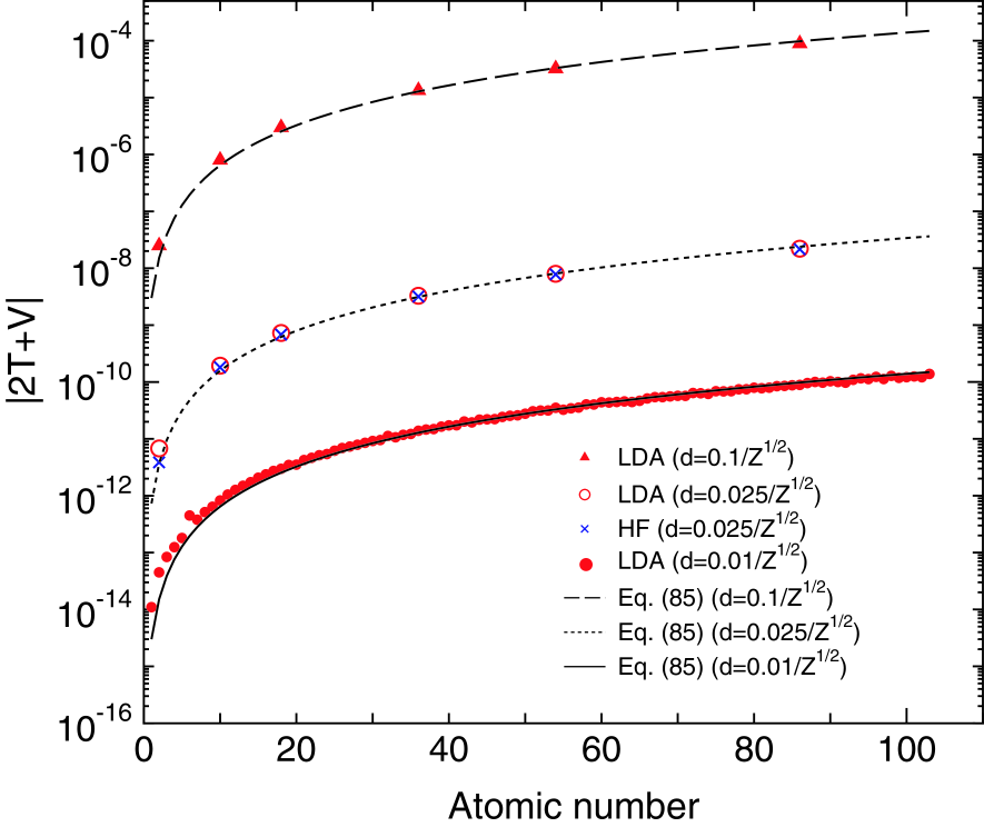
Figure: (Color online) The absolute value (hartree) of the virial theorem, $\vert 2T+V\vert$, as a function of atomic numbers calculated by the LDA and HF methods, and corresponding curves of error estimated by Eq. (85). The non-spin polarized ground state electronic configuration is considered for all the cases, and the spherical charge density distribution is assumed in the LDA calculations. The mesh spacing $d$ is taken to be $0.01/\sqrt {Z}$, $0.025/\sqrt {Z}$, $0.1/\sqrt {Z}$ bohr$^{1/2}$. $x_{\rm max}$ of 10 bohr$^{1/2}$ is used as the maximum range of $x$-coordinate for all the cases.

We now derive a formula which gives the absolute error in the total energy calculated by the FE method. In this derivation it is assumed that a large $x_{\rm max}$ is used so that the truncation of tail of wave functions cannot be a source of numerical error. The calculation in Fig. 2 suggests that $x_{\rm max}$ of 10 bohr$^{1/2}$ is large enough to avoid the error for all the elements (Z=1-103) in the periodic table. From the two observations that the error decreases algebraically as the mesh spacing decreases in Table I, and that the number of accurate digits of the total energy is nearly constant when the mesh spacing is taken to be inversely proportional to $\sqrt{Z}$, the number of accurate digits of the total energy, $N_{\rm d}$, may be written as

$$N_{\rm d} = a\log_{10}\left(\sqrt{Z}d\right) + b,$$ (78)

where $a$ and $b$ are parameters to be fitted, and $d$ is the mesh spacing as discussed before. Even if we have the same number of accurate digits of the total energy for different elements, the absolute error in the total energy depends on the absolute magnitude of the total energy. Therefore, as the next step, let us roughly estimate the total energy of atoms. Suppose that the total energy can be estimated by the sum of eigenvalues of hydrogen like atoms. Then, the total energy of an atom in which electrons fully occupy all the states up to the principal quantum number $n_{\rm max}$ is obtained by

$$E \propto \sum_{n=1}^{n_{\rm max}} \sum_{l=0}^{n-1}(2l+1)(-\frac{Z^2}{n^2}) = -n_{\rm max}Z^2.$$ (79)

In the case, the atomic number $Z$ is calculated by

$$Z = \sum_{n=1}^{n_{\rm max}} \sum_{l=0}^{n-1}2(2l+1),$$

$$= \frac{2}{3}n_{\rm max}^{3}+n_{\rm max}^{2}+\frac{1}{3}n_{\rm max}$$ (80)

which gives $n_{\rm max}\propto Z^{1/3}$ as $Z$ increases. Substituting the asymptotic form $n_{\rm max}\propto Z^{1/3}$ for Eq. (82), we have

$$E \propto -Z^{7/3}.$$ (81)

Noting that the number of accurate decimal places is given by $N_{\rm d}-\log_{10}\vert E\vert$, and using Eqs. (81) and (84), one can derive the following expression to estimate the absolute error, $E_{\rm err}$, in the total energy,

$$E_{\rm err} = 10^{-(N_{\rm d}-\log_{10}\vert E\vert)},$$

$$= \frac{\alpha Z^{7/3}}{10^b(\sqrt{Z}d)^a},$$ (82)

where $a$, $b$, and $\alpha$ are found to be -6, 2, and 0.3 by fitting Eq. (85) to the data shown in Fig. 2. As shown in Fig. 2 the estimated error by Eq. (85) fits well with that in the whole range we study. Strictly speaking, the expression of Eq. (85) estimates the error in the the virial theorem, since the fitting is done using the virial theorem $\vert 2T+V\vert$. However, the expression can be used to estimate the error in the total energy due to the near equivalence of the error between the virial theorem and the total energy. The expression implies that the error in the total energy approximately scales as $Z^{16/3}$ or $d^6$ when $d$ or $Z$ are fixed.

As well as the convergence property of the total energy, the eigenvalue of $1s$ state and the charge density at the origin in the ground state of a helium atom are shown as a function of the number of meshes in Table II. Although these quantities slowly converge compared to the total energy shown in Table I, it can be seen that the systematic convergence produces highly accurate results for both the LDA and HF calculations.

Table 2: The eigenvalue (hartree) of 1s state and charge density at the origin in the ground state of a helium atom. $x_{\rm max}$ of 10 bohr$^{1/2}$ is used as the maximum range of $x$-coordinate. The bold font means that the number is exact.

Meshes	Eigenvalue of $1s$		$n$ at the origin
		LDA
10	-0.471608882934828		4.5260991473798461147
20	-0.570859970667500		3.5721180605164599170
40	-0.570412462140008		3.5237334305245833802
80	-0.570424629988695		3.5258950648066678425
160	-0.570424750048491		3.5267674469147037484
320	-0.570424730001095		3.5268447250668697409
640	-0.570424724176759		3.5268499263432255490
1280	-0.570424722705590		3.5268502577049796584
		HF
10	-0.917364393558815		4.6752954006527842707
20	-0.917885224607414		3.6462035714690724058
40	-0.917953892393717		3.5931129688148539896
80	-0.917955530938917		3.5949601670283128317
160	-0.917955562327678		3.5958316993332024767
320	-0.917955562848009		3.5959123561764878905
640	-0.917955562856210		3.5959178873966144104
1280	-0.917955562856337		3.5959182401606711429

CONCLUSIONS

We have developed an accurate FE method for atomic calculations based on DFT within LDA and the Hartree-Fock method. Cubic Hermite spline functions on a uniform mesh for $x=\sqrt{r}$ are used as basis functions to expand the radial wave functions. The numerical integrations being a source of numerical error can be avoided due to the simplicity of the cubic Hermite spline functions, and all the associated integrals are analytically evaluated in conjunction with fitting of the hartree and exchange-correlation potentials to the same cubic Hermite spline functions. By taking account of the localized nature of the basis functions in real space, the generalized eigenvalue problem is efficiently solved using a generalized shift-invert iterative method for not only the LDA but also HF calculations. The numerical calculations show that the convergence is systematically controlled by the mesh spacing and in practice numerically exact solutions can be obtained within machine precision for all the elements (Z=1-103) in the periodic table. The convergence of the total energy from above implies that the FE method can be regarded as a variational scheme with respect to the Hermite spline functions for both the LDA and HF methods. Based on the virial theorem and an intuitive analysis the absolute error in the total energy is estimated to be proportional to $Z^{16/3}/d^6$. The absolute error is less than $10^{-7}$ hartree for the LDA and HF calculations when the mesh spacing $d$ is taken to be $0.025/\sqrt {Z}$ bohr$^{1/2}$. Since the FE method can provide high quality numerical solutions with a similar degree of accuracy for both DFT and the HF method, this can be utilized as a platform, which is free from the non-intrinsic numerical error in the validation of newly developed methods, for development of new functionals in DFT such as hybrid functionals. Along this line, we have been trying to develop a hybrid exchange hole model based on the FE method, which will be discussed elsewhere.

ACKNOWLEDGMENT

The authors were partly supported by the Fujitsu lab., the Nissan Motor Co., Ltd., Nippon Sheet Glass Co., Ltd., and the Next Generation Super Computing Project, Nanoscience Program, MEXT, Japan.

Bibliography

1

J.C. Slater, Quantum Theory of Atomic Structure, Vol. 1, McGraw-Hill, New York, 1960.

2

J.C. Slater, Quantum Theory of Atomic Structure, Vol. 2, McGraw-Hill, New York, 1960.

3

D. Feller, K.A. Peterson, and T.D. Crawford, J. Chem. Phys. 124 (2006) 054107.

4

R.M. Martin, Electronic Structure: Basic Theory and Practical Methods, Cambridge University Press, New York, 2008.

5

T. Helgaker, P. Jorgensen, and J. Olsen, Molecular Electronic-Structure Theory, Wiley, 2000.

6

C.E. Dykstra, G. Frenking, K.S. Kim, and G.E. Scuseria, Theory and Applications of Computational Chemistry: The First 40 Years (A Volume of Technical and Historical Perspectives), Elsevier, Amsterdam (2005).

7

B.W. Shore, J. Chem. Phys. 58 (1973) 3855.

8

J.L. Gázquez and H.J. Silverstone, J. Chem. Phys. 67 (1977) 1887.

9

C.F. Fischer and W. Guo, J. Comp. Phys. 90 (1990) 486.

10

H.T. Jeng and C.S. Hsue, Chin. J. Phys. 35 (1997) 215.

11

Z. Romanowski, Modelling Simul. Mater. Sci. Eng. 16, 015003 (2008); ibid. 17 (2009) 045001.

12

D. Engel, M. Klews, and G. Wunner, Comp. Phys. Comm. 180 (2009) 302.

13

S.R. White, J.W. Wilkins, and M.P. Teter, Phys. Rev. B 39 (1989) 5819.

14

E. Tsuchida and M. Tsukada, Phys. Rev. B 54 (1996) 7602.

15

J.E. Pask and P. Sterne, Modelling Simul. Mater. Sci. Eng. 13 (2005) R71.

16

E.J. Bylaska, M. Holst, and J.H. Weare, J. Chem. Theory Comput. 5 (2009) 937.

17

P. Hohenberg and W. Kohn, Phys. Rev. 136 (1964) B864.

18

W. Kohn and L. J. Sham, Phys. Rev. 140 (1965) A1133.

19

A.D. Becke, J. Chem. Phys. 98 (1993) 1372.

20

T. Leininger, H. Stoll, H.-J. Werner, and A. Savin, Chem. Phys. Lett. 275 (1997) 151.

21

H. Iikura, T. Tsuneda, T. Yanai, and K. Hirao, J. Chem. Phys. 115 (2001) 3540.

22

J. Heyd, G.E. Scuseria, and M. Ernzerhof, J. Chem. Phys. 118 (2003) 8207.

23

T.M. Henderson, A.F. Izmaylov, G. Scalmani, and G.E. Scuseria, J. Chem. Phys. 131 (2009) 044108.

24

In addition to the change of variables, $r = x^2$, we tried two other cases, $r=\exp(x)$ and $r=\exp(x^2)-1$, and found that the latter two cases lead to complication in the formalism.

25

D.M. Ceperley and B.J. Alder, Phys. Rev. Lett. 45 (1980) 566.

26

S.H. Vosko, L. Wilk, and M. Nusair, Can. J. Phys. 58, (1980) 1200; S.H. Vosko and L. Wilk, Phys. Rev. B 22, (1980) 3812.

27

J.P. Perdew, K. Burke, and M. Ernzerhof, Phys. Rev. Lett. 77 (1996) 3865.

28

In addition to the cubic Hermite spline functions, we investigated the convergence of the quintic Hermite spline functions, and found that the convergence ratio with respect to the total number of basis functions is comparable to the cubic case. Thus, it is concluded that the cubic Hermite spline functions is an optimum choice with respect to the convergence ratio and the simplicity of analytic expressions derived for matrix elements.

29

Z. Bai, J. Demmel, J. Dongarra, A. Ruhe, and H. van der Vorst, Templates for the Solution of Algebraic Eigenvalue Problems: A Practical Guide, Society for Industrial Mathematics (1987).

30

F.W. Averill and G.S. Painter, Phys. Rev. B 24 (1981) 6795.

31

J.C. Slater, J. Chem. Phys. 57 (1972) 2389.

32

The total energy we obtain corresponds to that in the nonrelativistic HF limit, which lacks the correlation energy of -0.042044 hartree compared to the exact energy of -2.903724 hartree.

33

The program code, ADPACK, and the calculated results are available on a web site (http://www.openmx-square.org/).

34

S. Kotochigova, Z.H. Levine, E.L. Shirley, M.D. Stiles, and C.W. Clark, Phys. Rev. A 55, 191 (1997); a web site of the database
(http://www.nist.gov/physlab/data/dftdata/)