Efficient low-order scaling method for large-scale electronic structure calculations with localized basis functions: Ver. 1.0
The original has been published in Phys. Rev. B 82, 075131 (2010).

Abstract

An efficient low-order scaling method is presented for large-scale electronic structure calculations based on the density functional theory using localized basis functions, which directly computes selected elements of the density matrix by a contour integration of the Green function evaluated with a nested dissection approach for resultant sparse matrices. The computational effort of the method scales as O($N{({\log }_{2}N)}^2$), O($N^2$), and O($N^{7/3}$) for one, two, and three dimensional systems, respectively, where $N$ is the number of basis functions. Unlike O($N$) methods developed so far the approach is a numerically exact alternative to conventional O($N^3$) diagonalization schemes in spite of the low-order scaling, and can be applicable to not only insulating but also metallic systems in a single framework. It is also demonstrated that the well separated data structure is suitable for the massively parallel computation, which enables us to extend the applicability of density functional calculations for large-scale systems together with the low-order scaling.

1 INTRODUCTION

During the last three decades continuous efforts [3, 4, 5, 6, 7, 8, 9, 10, 11, 12, 13, 14, 15, 16, 17, 18, 19, 21, 20, 22, 23, 24, 25, 26, 27, 28, 29, 30, 31] have been devoted to extend applicability of the density functional theory (DFT)[1, 2] to large-scale systems, which leads to realization of more realistic simulations being close to experimental conditions. In fact, lots of large-scale DFT calculations have already contributed for comprehensive understanding of a vast range of materials,[32, 33, 34, 35, 36, 37] although widely used functionals such as local density approximation (LDA)[38] and generalized gradient approximation (GGA)[39] have limitation in describing strong correlation in transition metal oxides and van der Waals interaction in biological systems.

The efficient methods developed so far within the conventional DFT can be classified into two categories in terms of computational complexity, [3, 4, 5, 6, 7, 8, 9, 10, 11, 12, 13, 14, 15, 16, 17, 18, 19, 21, 20, 22, 23, 24, 25, 26, 27, 28] while the other methods, which deviate from the classification, have been also proposed.[29, 30, 31] The first category consists of O($N^3$) methods, [3, 4, 5, 6, 7, 8, 9, 10, 11, 12] where $N$ is the number of basis functions, as typified by the Householder-QR method,[11, 12] the conjugate gradient method,[4, 8, 9] and the Pulay method,[6, 7] which have currently become standard methods. The methods can be regarded as numerically exact methods, and the computational cost scales as O($N^3$) even if only valence states are calculated because of the orthonormalization process. On the other hand, the second category involves approximate O($N$) methods such as the density matrix methods,[21, 22, 23] the orbital minimization methods,[20, 25] and the Krylov subspace methods[16, 17, 18, 19, 27] of which computational cost is proportional to the number of basis functions $N$. The linear-scaling of the computational effort in the O($N$) methods can be achieved by introducing various approximations like the truncation of the density matrix[21] or Wannier functions[20, 25] in real space. Although the O($N$) methods have been proven to be very efficient, the applications must be performed with careful consideration due to the introduction of the approximations, which might be one of reasons that the O($N$) methods have not been widely used compared to the O($N^3$) methods. From the above reason one may think of whether a numerically exact but low-order scaling method can be developed by utilizing the resultant sparse structure of the Hamiltonian and overlap matrices expressed by localized basis functions. Recently, a direction towards the development of O($N^{2\sim }$) methods has been suggested by Lin et al., in which diagonal elements of the density matrix is computed by a contour integration of the Green function calculated by making full use of the sparse structure of the matrix.[40] Also, efficient schemes have been developed to calculate certain elements of the Green function for electronic transport calculations,[41, 42] which are based on the algorithm by Takahashi et al.[43] and Erisman and Tinney.[44] However, except for the methods mentioned above the development of numerically exact O($N^{2\sim }$) methods, which are positioned in between the O($N$) and O($N^3$) methods, has been rarely explored yet for large-scale DFT calculations.[45]

In this paper we present a numerically exact but low-order scaling method for large-scale DFT calculations of insulators and metals using localized basis functions such as pseudo-atomic orbital (PAO),[46] finite element (FE),[47] and wavelet basis functions.[48] The computational effort of the method scales as O($N{({\log }_{2}N)}^2$), O($N^2$), and O($N^{7/3}$) for one, two, and three dimensional (1D, 2D, and 3D) systems, respectively. In spite of the low-order scaling, the method is a numerically exact alternative to the conventional O($N^3$) methods. The key idea of the method is to directly compute selected elements of the density matrix by a contour integration of the Green function evaluated with a set of recurrence formulas. It is shown that a contour integration method based on a continued fraction representation of the Fermi-Dirac function[49] can be successfully employed for the purpose, and that the number of poles used in the contour integration does not depend on the size of the system. We also derive a set of recurrence formulas based on the nested dissection[51] of the sparse matrix and a block $LD{L}^T$ factorization using the Schur complement[12] to calculate selected elements of the Green function. The computational complexity is governed by the calculation of the Green function. In addition to the low-order scaling, the method can be particularly advantageous to the massively parallel computation because of the well separated data structure.

This paper is organized as follows: In Sec. 2 the theory of the proposed method is presented together with detailed analysis of the computational complexity. In Sec. 3 several numerical calculations are shown to illustrate practical aspects of the method within a model Hamiltonian and DFT calculations using the PAO basis functions. In Sec. 4 we summarize the theory and applicability of the numerically exact but low-order scaling method.

2 THEORY

2.1 Density matrix approach

Let us assume that the Kohn-Sham (KS) orbital ${\varphi }_{\nu }$ is expressed by a linear combination of localized basis functions $\{\chi \}$ such as PAO,[46] FE,[47] and wavelet basis functions[48] as:

${\varphi }_{\nu }(𝐫)={\displaystyle \sum _{i=1}^N}{c}_{\nu i}{\chi }_i(𝐫),$ (1)

where $N$ is the number of basis functions. Throughout the paper, we consider the spin restricted and $𝐤$-independent KS orbitals for simplicity of notation. However, the generalization of our discussion for these cases is straightforward. By introducing LDA or GGA for the exchange-correlation functional, the KS equation is written in a sparse matrix form:

$H{c}_{\nu }={\epsilon }_{\nu }S{c}_{\nu },$ (2)

where ${\epsilon }_{\nu }$ is the eigenvalue of state $\nu$, $c_{\nu }$ a vector consisting of coefficients $\{c_{\nu i}\}$, and $H$ and $S$ are the Hamiltonian and overlap matrices, respectively. Due to both the locality of basis functions and LDA or GGA for the exchange-correlation functional, both the matrices possess the same sparse structure. It is also noted that the charge density $n(𝐫)$ can be calculated by the density matrix $\rho$:

$n(𝐫)={\displaystyle \sum _{i,j}}{\rho }_{ij}{\chi }_j(𝐫){\chi }_i(𝐫).$ (3)

By remembering that $\chi$ is localized in real space, one may notice that the product ${\chi }_i{\chi }_j$ is non-zero only if they are closely located each other. Thus, the number of elements in the density matrix required to calculate the charge density scales as O($N$). As well as the calculation of the charge density, the total energy is computed by only the corresponding elements of the density matrix within the conventional DFT as:

$E_{\mathrm{tot}}[n,\rho ]$ $=$ $\mathrm{Tr}(\rho H_{\mathrm{kin}})+{\displaystyle \int 𝑑𝐫n(𝐫)v_{\mathrm{ext}}(𝐫)}+{\displaystyle \int \int 𝑑𝐫𝑑{𝐫}^{\prime }\frac{n(𝐫)n({𝐫}^{\prime })}{|𝐫-{𝐫}^{\prime }|}}+E_{\mathrm{xc}}[n],$ (4)

where $H_{\mathrm{kin}}$ is the matrix for the kinetic operator, $v_{\mathrm{ext}}$ an external potential, and $E_{\mathrm{xc}}$ an exchange-correlation functional. Since the matrix $H_{\mathrm{kin}}$ possesses the same sparse structure as that of $S$, one may find an alternative way that the selected elements of the density matrix, corresponding to the non-zero products ${\chi }_i{\chi }_j$, are directly computed without evaluating the KS orbitals. The alternative way enables us to avoid an orthogonalization process such as Gram-Schmidt method for the KS orbitals, of which computational effort scales as O($N^3$) even if only the occupied states are taken into account. The direct evaluation of the selected elements in the density matrix is the starting point of the method proposed in the paper. In this sense, the low-order scaling method is similar to O($N$) Green funtion methods such as recursion and bond-order potential methods,[16, 17, 18] while the Green function is approximately evaluated in these O($N$) methods. The density matrix $\rho$ can be calculated through the Green function $G$ as follows:

$\rho =-{\displaystyle \frac{2}{\pi }}\mathrm{Im}{\displaystyle {\int }_{-\mathrm{\infty }}^{\mathrm{\infty }}}𝑑EG(E+i{0}^{+})f\left({\displaystyle \frac{E-\mu }{k_{\mathrm{B}}T}}\right),$ (5)

where the factor 2 is due to the spin degeneracy, $f$ the Fermi-Dirac function, $\mu$ chemical potential, $T$ electronic temperature, $k_{\mathrm{B}}$ the Boltzmann factor, and $0^{+}$ a positive infinitesimal. Also the matrix expression of the Green function is given by

$G(Z)={(ZS-H)}^{-1},$ (6)

where $Z$ is a complex number. Therefore, from Eqs. (5) and (6), our problem is cast to two issues: (i) how the integration of the Green function can be efficiently performed, and (ii) how the selected elements of the Green function in the matrix form can be efficiently evaluated. In the subsequent subsections we discuss the two issues in detail.

2.2 Contour integration of the Green function

We perform the integration of the Green function, Eq. (5), by a contour integration method using a continued fraction representation of the Fermi-Dirac function.[49] In the contour integration the Fermi-Dirac function is expressed by

${\displaystyle \frac{1}{1+\exp (x)}}$ $=$ ${\displaystyle \frac{1}{2}}-{\displaystyle \frac{\frac{x}{4}}{1+{\displaystyle \frac{{(\frac{x}{2})}^2}{3+{\displaystyle \frac{{(\frac{x}{2})}^2}{5+{\displaystyle \frac{{(\frac{x}{2})}^2}{{{\displaystyle \frac{\mathrm{\cdots }}{(2M-1)+}}}_{\mathrm{\ddots }}}}}}}}}}$ (7)

$=$ ${\displaystyle \frac{1}{2}}+{\displaystyle \sum _{p=1}^{\mathrm{\infty }}}{\displaystyle \frac{R_p}{x-i{z}_p}}+{\displaystyle \sum _{p=1}^{\mathrm{\infty }}}{\displaystyle \frac{R_p}{x+i{z}_p}},$

where $x=\beta (Z-\mu )$ with $\beta =\frac{1}{k_{\mathrm{B}}T}$, $z_p$ and $R_p$ are poles of the continued fraction representation and the associated residues, respectively. The representation of the Fermi-Dirac function is derived from a hypergeometric function, and can be regarded as a Padé approximant when terminated at the finite continued fraction. The poles $z_p$ and residues $R_p$ can be easily obtained by solving an eigenvalue problem as shown in Ref. [49]. By making use of the expression of Eq. (7) for Eq. (5) and considering the contour integration, one obtain the following expression for the integration of Eq. (5):

$\rho$ $=$ $M^{(0)}+\mathrm{Im}\left(-{\displaystyle \frac{4i}{\beta }}{\displaystyle \sum _{p=1}^{\mathrm{\infty }}}G({\alpha }_p)R_p\right),$ (8)

where ${\alpha }_p=\mu +i\frac{z_p}{\beta }$, and $M^{(0)}$ is the zeroth order moment of the Green function which can be computed by $i{R}_{\mathrm{d}}G(i{R}_{\mathrm{d}})$ with a large real number $R_{\mathrm{d}}$ of ${10}^{10}$ Hartree. The structure of the poles distribution, that all the poles are located on the imaginary axis like the Matsubara pole, but the density of the poles becomes smaller as the poles go away from the real axis, has been found to be very effective for the efficient integration of Eq. (5). It has been shown that only the use of the 100 poles at 600 K gives numerically exact results within double precision.[49] Thus, the contour integration method can be regarded as a numerically exact method even if the summation is terminated at a practically modest number of poles.

Moreover, it should be noted that the number of poles to achieve convergence is independent of the size of system. Giving the Green function in the Lehmann representation, Eq. (8) can be rewritten by

$\rho$ $=$ $M^{(0)}+\mathrm{Im}\left(-{\displaystyle \frac{4i}{\beta }}{\displaystyle \sum _{p=1}^{\mathrm{\infty }}}{\displaystyle \sum _{\nu }}{\displaystyle \frac{|{\varphi }_{\nu }⟩⟨{\varphi }_{\nu }|}{{\alpha }_p-{\epsilon }_{\nu }}}{R}_p\right)$ (9)

$=$ $M^{(0)}+{\displaystyle \sum _{\nu }}\mathrm{Im}\left(-{\displaystyle \frac{4i}{\beta }}{\displaystyle \sum _{p=1}^{\mathrm{\infty }}}{\displaystyle \frac{|{\varphi }_{\nu }⟩⟨{\varphi }_{\nu }|}{{\alpha }_p-{\epsilon }_{\nu }}}{R}_p\right).$

Although the expression in the second line is obtained by just exchanging the order of the two summations, the expression clearly shows that the number of poles for convergence does not depend on the size of system if the spectrum radius is independent of the size of system. Since the independence of the spectrum radius can be found in general cases, it can be concluded that the computational effort is determined by that for the calculation of the Green function.

The energy density matrix $e$, which is needed to calculate forces on atoms within non-orthogonal localized basis functions, can also be calculated by the contour integration method[49] as follows:

$e$ $=$ $-{\displaystyle \frac{2}{\pi }}\mathrm{Im}{\displaystyle {\int }_{-\mathrm{\infty }}^{\mathrm{\infty }}}𝑑EEG(E+i{0}^{+})f\left({\displaystyle \frac{E-\mu }{k_{\mathrm{B}}T}}\right),$ (10)

$=$ $M^{(1)}+\kappa M^{(0)}+\mathrm{Im}\left(-{\displaystyle \frac{4i}{\beta }}{\displaystyle \sum _{p=1}^{\mathrm{\infty }}}G({\alpha }_p)R_p{\alpha }_p\right)$

with $\kappa$ defined by

$\kappa ={\displaystyle \frac{4}{\beta }}{\displaystyle \sum _{p=1}^{\mathrm{\infty }}}{R}_p,$ (11)

where $M^{(0)}$ and $M^{(1)}$ are the the zeroth and first order moments of the Green function, and can be computed by solving the following simultaneous linear equation:

(12)

The equation is derived by terminating the summation over the order of the moments in the moment representation of the Green function. By letting $z_0$ and $z_1$ be $i{R}_{\mathrm{e}}^2$ and $i{R}_{\mathrm{e}}$, [50] respectively, $M^{(0)}$ and $M^{(1)}$ are explicitly given by

$M^{(0)}$ $=$ ${\displaystyle \frac{i{R}_{\mathrm{e}}}{R_{\mathrm{e}}-1}}\left(R_{\mathrm{e}}^{2}G(i{R}_{\mathrm{e}}^2)-G(i{R}_{\mathrm{e}})\right),$ (13)

$M^{(1)}$ $=$ ${\displaystyle \frac{R_{\mathrm{e}}^3}{R_{\mathrm{e}}-1}}\left(R_{\mathrm{e}}G(i{R}_{\mathrm{e}}^2)-G(i{R}_{\mathrm{e}})\right),$ (14)

where $R_{\mathrm{e}}$ should be a large real number, and ${10}^7$ Hartree is used in this study so that the higher order terms can be negligible in terminating the summation in the moment representation of the Green function. Inserting Eqs. (13) and (14) into Eq. (10), we obtain the following expression which is suitable for the efficient implementation in terms of memory consumption:

$e$ $=$ $\lambda G(i{R}_{\mathrm{e}}^2)+\gamma G(i{R}_{\mathrm{e}})+\mathrm{Im}\left(-{\displaystyle \frac{4i}{\beta }}{\displaystyle \sum _{p=1}^{\mathrm{\infty }}}G({\alpha }_p)R_p{\alpha }_p\right)$ (15)

with $\lambda$ and $\gamma$ defined by

$\lambda$ $=$ ${\displaystyle \frac{R_{\mathrm{e}}^3}{R_{\mathrm{e}}-1}}(R_{\mathrm{e}}+i\kappa ),$ (16)

$\gamma$ $=$ $-{\displaystyle \frac{R_{\mathrm{e}}}{R_{\mathrm{e}}-1}}(R_{\mathrm{e}}^2+i\kappa ).$ (17)

One may notice that the number of poles for convergence does not depend on the size of system even for the calculation of the energy density matrix because of the same reason as for the density matrix.

2.3 Calculation of the Green function

It is found from the above discussion that the computational effort to compute the density matrix is governed by that for the calculation of the Green function, consisting of an inversion of the sparse matrix of which computational effort by conventional schemes such as the Gauss elimination or LU factorization based methods scales as O($N^3$). Thus, the development of an efficient method of inverting a sparse matrix is crucial for efficiency of the proposed method.

Here we present an efficient low-order scaling method, based on a nested dissection approach,[51] of computing only selected elements in the inverse of a sparse matrix. The low-order scaling method proposed here consists of two steps: (1) Nested dissection: by noting that a matrix $X\equiv (ZS-H)$ is sparse, a structured matrix is constructed by a nested dissection approach. In practice, just reordering the column and row indices of the matrix $X$ yields the structured matrix. (2) Inverse by recurrence formulas: by recursively applying a block $LD{L}^T$ factorization[12] to the structured matrix, a set of recurrence formulas is derived. Using the recurrence formulas, only the selected elements of the inverse matrix $X^{-1}\equiv G(Z)$ are directly computed. The computational effort to calculate the selected elements in the inverse matrix using the steps (i) and (ii) scales as O($N{({\log }_{2}N)}^2$), O($N^2$), and O($N^{7/3}$) for 1D, 2D, and 3D systems, respectively, as shown later. First, we discuss the nested dissection of a sparse matrix, and then derive a set of recurrence formulas of calculating the selected elements of the inverse matrix.

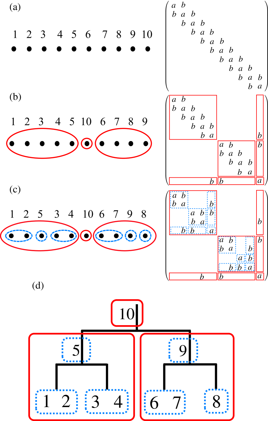
Figure 1: (Color online) (a) The initial numbering for atoms in a linear chain molecule consisting of ten atoms described by the $s$-valent NNTB and its corresponding matrix, (b) the renumbering for atoms by the first step in the nested dissection and its corresponding matrix, (c) the renumbering for atoms by the second step in the nested dissection and its corresponding matrix, (d) the binary tree structure representing hierarchical interactions between domains in the structured matrix by the numbering shown in Fig. 1(c).

2.3.1 Nested dissection

As an example the right panel of Fig. 1(c) shows a structured matrix obtained by the nested dissection approach for a finite chain model consisting of ten atoms, where we consider a $s$-valent nearest neighbor tight binding (NNTB) model. When one assigns the number to the ten atoms as shown in the left panel of Fig. 1(a), then $X$ is a tridiagonal matrix, of which diagonal and off-diagonal terms are assumed to be $a$ and $b$, respectively, as shown in the right panel of Fig. 1(a). As the first step to generate the structured matrix shown in the right panel of Fig. 1(c), we make a dissection of the system into the left and right domains[52] by renumbering for the ten atoms, and obtain a dissected matrix shown in the right panel of Fig. 1(b). The left and right domains interact with each other through only a separator consisting of an atom 10. As the second step we apply a similar dissection for each domain generated by the first step, and arrive at a nested-dissected matrix given by the right panel of Fig. 1(c). The subdomains, which consist of atoms 1 and 2 and atoms 3 and 4, respectively, in the left domain interact with each other through only a separator consisting of an atom 5. The similar structure is also found in the right domain consisting of atoms 6, 7, 9, and 8. It is worth mentioning that the resultant nested structure of the sparse matrix can be mapped to a binary tree structure which indicates hierarchical interactions between (sub)domains as shown in Fig. 1(d). By applying the above procedure to a sparse matrix, one can convert any sparse matrix into a nested and dissected matrix in general. However in practice there is no obvious way to perform the nested dissection for general sparse matrices, while a lot of efficient and effective methods have been already developed for the purpose.[53, 54] Here we propose a rather simple but effective way for the nested dissection by taking account of a fact that the basis function we are interested in is localized in real space, and that the sparse structure of the resultant matrix is very closely related to the position of basis functions in real space. The method bisects a system into two domains interacting through only a separator, and recursively applies to the resultant subdomains, leading to a binary tree structure for the interaction. Our algorithm for the nested dissection of a general sparse matrix is summarized as follows:

(i) Ordering. Let us assume that there are $N_d$ basis functions in a domain we are interested in. We order the basis functions in the domain by using the fractional coordinate for the central position of localized basis functions along ${𝐚}_i$-axis, where $i=1,2$, and 3. As a result of the ordering, each basis function can be specified by the ordering number, which runs from 1 to $N_d$ in the domain of the central unit cell. The ordering number in the periodic cells specified by $l{𝐚}_i$, where $l=0,\pm 1,\pm 2,\mathrm{\cdots }$, is given by $l{N}_d+q$, where $q$ is the corresponding ordering number in the central cell. In isolated systems, one can use the Cartesian coordinate instead of the fractional coordinate without losing any generality.

(ii) Screening of basis functions with a long tail. The basis functions with a long tail tend to make an efficient dissection difficult. The sparse structure formed by the other basis functions with a short tail hides behind the dense structure caused by the basis functions with a long tail. Thus, we classify the basis functions with a long tail in the domain as members in the separator before performing the dissection process. By the screening of the basis functions with a long tail, it is possible to expose concealed sparse structure when atomic basis functions with a variety of tails are used, while a systematic basis set such as the FE basis functions may not require the screening.

(iii) Finding of a starting nucleus. Among the localized basis functions in the domain, we search a basis function which has the smallest number of non-zero overlap with the other basis functions. Once the basis function is found, we set it as a starting nucleus of a subdomain.

(iv) Growth of the nucleus. Staring from a subdomain (nucleus) given by the procedure (iii), we grow the subdomain by increasing the size of nucleus step by step. The growth of the nucleus can be easily performed by managing the minimum and maximum ordering numbers, $m_{\min }$ and $m_{\max }$, which ranges from 1 to $N_d$, and the grown subdomain is defined by basis functions with the successive ordering numbers between the minimum and maximum ordering numbers $m_{\min }$ and $m_{\max }$. At each step in the growth of the subdomain, we search two basis functions which have the minimum ordering number $n_{\min }$ and maximum ordering number $n_{\max }$ among basis functions overlapping with the subdomain defined at the growth step. In the periodic boundary condition, $n_{\min }$ can be smaller than zero, and $n_{\max }$ can be larger than the number of basis functions $N_d$. Then, the number of basis functions in the subdomain, the separator, and the other subdomain can be calculated by $N_0\equiv m_{\max }-m_{\min }+1$, $N_{\mathrm{s}}\equiv n_{\max }-n_{\min }+1-N_0$, and $N_1\equiv N_d-N_0-N_{\mathrm{s}}$, respectively, at each growth step. By the growth process one can minimize $(|N_0-N_1|+N_{\mathrm{s}})$ being a measure for quality of the dissection, where the measure $(|N_0-N_1|+N_{\mathrm{s}})$ takes equal bisection size of the subdomains and minimization of the size of the separator into account. Also if $(n_{\max }-n_{\min }+1)$ is larger than $N_d$, then this situation implies that the proper dissection can be difficult along the axis.

(v) Dissection. By applying the above procedures (i)-(iv) to each ${𝐚}_i$-axis, where $i=1,2$, and 3, and we can find an axis which gives the minimum $(|N_0-N_1|+N_{\mathrm{s}})$. Then, the dissection along the axis is performed by renumbering for basis functions in the domain, and two subdomains and one separator are obtained. Evidently, the same procedures can be applied to each subdomain, and recursively continued until the size of domain reaches a threshold. As a result of the recursive dissection, a structured matrix specified by a binary tree is obtained.

As an illustration we apply the method for the nested dissection to the finite chain molecule shown in Fig. 1. We first set all the system as domain, and start to apply the series of procedures to the domain. The procedure (i) is trivial for the case, and we obtain the numbering of atoms and the corresponding matrix shown in Fig. 1(a). Also it is noted that the screening of the basis functions with a long tail is unnecessary, and that we only have to search the chain direction. In the procedure (iii), atoms 1 and 10 in Fig. 1(a) satisfy the condition. Choosing the atom 1 as a starting nucleus of the domain, and we gradually increase the size of the domain according to the procedure (iv). Then, it is found that the division shown in Fig. 1(b) gives the minimum $(|N_0-N_1|+N_{\mathrm{s}})$. Renumbering for the basis functions based on the analysis yields the dissected matrix shown in the right panel of Fig. 1(b). By applying the similar procedures to the left and right subdomains, one will immediately find the result of Fig. 1(c).

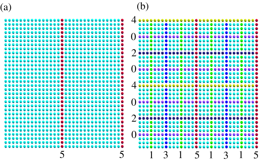
Figure 2: (Color online) (a) The square lattice model, described by the $s$-valent NNTB, of which unit cell contains 1024 atoms with periodic boundary condition. The right blue and red circles correspond to atoms in two domains and a separator, respectively, at the first step in the nested dissection. (b) The square lattice model at the final step in the nested dissection. The separator at the innermost and the outermost levels are labeled as separators 0 and 5, respectively, and the separators at each level are constructed by atoms with a same color.

In addition to the finite chain molecule, as an example of more general cases, the above algorithm for the nested dissection is applied to a $s$-valent NNTB square lattice model of which unit cell contains 1024 atoms with periodic boundary condition. At the first step in the nested dissection, the separator is found to be red atoms as shown in Fig. 2(a). Due to the periodic boundary condition, the separator consists of two lines. At the final step, the system is dissected by the recursive algorithm as shown in Fig. 2(b). The separator at the innermost and the outermost levels are labeled as separators 0 and 5, respectively, and each subdomain at the innermost level includes 9 atoms. As demonstrated for the square lattice model, the algorithm can be applied for systems with any dimensionality, and provides a well structured matrix for our purpose in a single framework.

2.3.2 Inverse by recurrence formulas

We directly compute the selected elements of the inverse matrix using a set of recurrence formulas which can be derived by recursively applying a block $LD{L}^T$ factorization to the structured matrix obtained by the nested dissection method as shown below. To derive the recurrence formulas, we first introduce the block $LD{L}^T$ factorization[12] for a symmetric square matrix $X$:

$X$ $=$ (18)

$=$

where $A$ and $C$ are diagonal block matrices, and $B$ and $B^T$ an off-diagonal block matrix and its transposition, and $L$ is given by

$L=B{A}^{-1}.$ (19)

Also the Schur complement $S$ of the block element $C$ is defined by

$S\equiv C-B{A}^{-1}{B}^T=C-B{L}^T.$ (20)

Then, it is verified that the inverse matrix of $X$ is given by

(21)

We now consider calculating the selected elements of the inverse of the structured matrix given in Fig. 1(c) using Eq. (21), and rewrite the matrix in Fig. 1(c) in a block form as follows:

(22)

where $A_{0,0}$ and $B_{0,0}$ correspond to and $(0,b)$, respectively, and the other block elements can be deduced. Also the blank indicates a block zero element. Using Eq. (20) the Schur complement of $C_{1,0}$ is given by

$S_{1,0}=C_{1,0}-B_{1,0}{L}_{1,0}^T-B_{1,1}{L}_{1,1}^T,$ (23)

where $L_{1,0}^T$ is calculated by Eq. (19) and can be transformed using Eq. (21) to a recurrence formula as follows:

$L_{1,0}^T$ $=$ (24)

$=$

$=$ $\left(\begin{array}{c}\hfill V_{1,0,0}^T\hfill \\ \hfill V_{1,0,1}^T\hfill \\ \hfill 0\hfill \end{array}\right)+\left(\begin{array}{c}\hfill L_{0,0}^T\hfill \\ \hfill L_{0,1}^T\hfill \\ \hfill -I\hfill \end{array}\right)Q_{1,1,0}^T\equiv V_{1,1,0}^T$

with the definitions:

$V_{1,0,0}^T$ $=$ $A_{0,0}^{-1}{(B_{1,0}[B_{0,0}])}^T,$ (25)

$V_{1,0,1}^T$ $=$ $A_{0,1}^{-1}{(B_{1,0}[B_{0,1}])}^T,$ (26)

and

$Q_{1,1,0}^T=S_{0,0}^{-1}\left(B_{0,0}{V}_{1,0,0}^T+B_{0,1}{V}_{1,0,1}^T-{(B_{1,0}[C_{0,0}])}^T\right).$ (27)

In Eqs. (25), (26), and (27), we used a bra-ket notation [ ] which stands for a part of the block element. For example, $B_{1,0}[B_{0,0}]$ means a part of $B_{1,0}$ which has the same columns as those of $B_{0,0}$. It is noted that one can obtain a similar expression for $L_{1,1}^T$ as well as Eq. (24) for $L_{1,0}^T$.

To address a more general case where the dissection for the sparse matrix is further nested, we suppose that the matrix $A_{0,0}$ has the same inner structure as

then one may notice the recursive structure in Eq. (24), and can derive the following set of recurrence relations for general cases:

$Q_{p,m+1,n}^T$ $=$ $S_{m,n}^{-1}\left(B_{m,2n}{V}_{p,m,2n}^T+B_{m,2n+1}{V}_{p,m,2n+1}^T-{(B_{p,q}[C_{m,n}])}^T\right),$ (28)

$V_{p,m+1,n}^T$ $=$ $\left(\begin{array}{c}\hfill V_{p,m,2n}^T\hfill \\ \hfill V_{p,m,2n+1}^T\hfill \\ \hfill 0\hfill \end{array}\right)+\left(\begin{array}{c}\hfill L_{m,2n}^T\hfill \\ \hfill L_{m,2n+1}^T\hfill \\ \hfill -I\hfill \end{array}\right)Q_{p,m+1,n}^T.$ (29)

Equation (29) is the central recurrence formula coupled with Eq. (28), where the initial block elements are given by

$V_{p,0,n}^T={(A_{0,n})}^{-1}{(B_{p,q}[B_{0,n}])}^T.$ (30)

Also $L_{p,n}$ and $S_{p,n}$ can be calculated by

$L_{p,n}$ $=$ $V_{p,p,n},$ (31)

$S_{p,n}$ $=$ $C_{p,n}-(B_{p,2n},B_{p,2n+1})\left(\begin{array}{c}\hfill L_{p,2n}^T\hfill \\ \hfill L_{p,2n+1}^T\hfill \end{array}\right).$ (32)

A set of Eqs. (28)-(32) enables us to calculate all the inverses of the Schur complements $S$ and $L$. In the recurrence formulas Eqs. (28) and (29), three indices of $p$, $m$, and $n$ are involved, and they run as follows:

$p$ $=$ $0,\mathrm{\cdots },P.$ (33)

$m$ $=$ $0,\mathrm{\cdots },p-1.$ (34)

$n$ $=$ $0,\mathrm{\cdots },2^{P-m}-1.$ (35)

The index $p$ denotes the level of hierarchy in the nested dissection and the innermost and outermost levels are set to 0 and $P$, respectively. Then, it is noted that the total system is divided into $2^{P+1}$ domains at the innermost level. As well as $p$ the index $m$ is also related to the level of hierarchy in the nested dissection, and runs from 0 to $p-1$. The index $n$ is a rather intermediate one, being dependent on $m$. The indices $n$ in Eq. (30) is dependent on $p$ and $q$ and they run as follows:

$n$ $=$ $q(2^p),\mathrm{\cdots },(q+1)(2^p)-1.$ (36)

$q$ $=$ $0,\mathrm{\cdots },2^{P+1-p}-1.$ (37)

Since the set of the recurrence formulas Eqs. (28)-(32) proceed according to Eqs .(33)-(35), the development of recurrence can be illustrated as in Fig. 3. The recurrence starts from Eq. (30) with $p=0$, and Eqs. (31) and (32) follow. Then, $p$ is incremented by one, and $m+1$ climbs up to 1. The increment of $p$ and the climbing of $m+1$ are repeated until $p=P$ and $m+1=P$. At $m+1=p$ for each $p$, $L$ and $S$ are evaluated by Eqs. (31) and (32), and the inverse of $S$ is calculated by a conventional method such as LU factorization, which are used in the next recurrence for the higher level of hierarchy. The numbers in the right hand side of Fig. 3 give the multiplicity for similar calculations by Eq. (29) coming from the index $n$ at each $m+1$, since $n$ runs from 0 to $2^{P-m}-1$ as given in Eq. (35). The computational complexity can be estimated by Fig. 3, and we will discuss its details later.

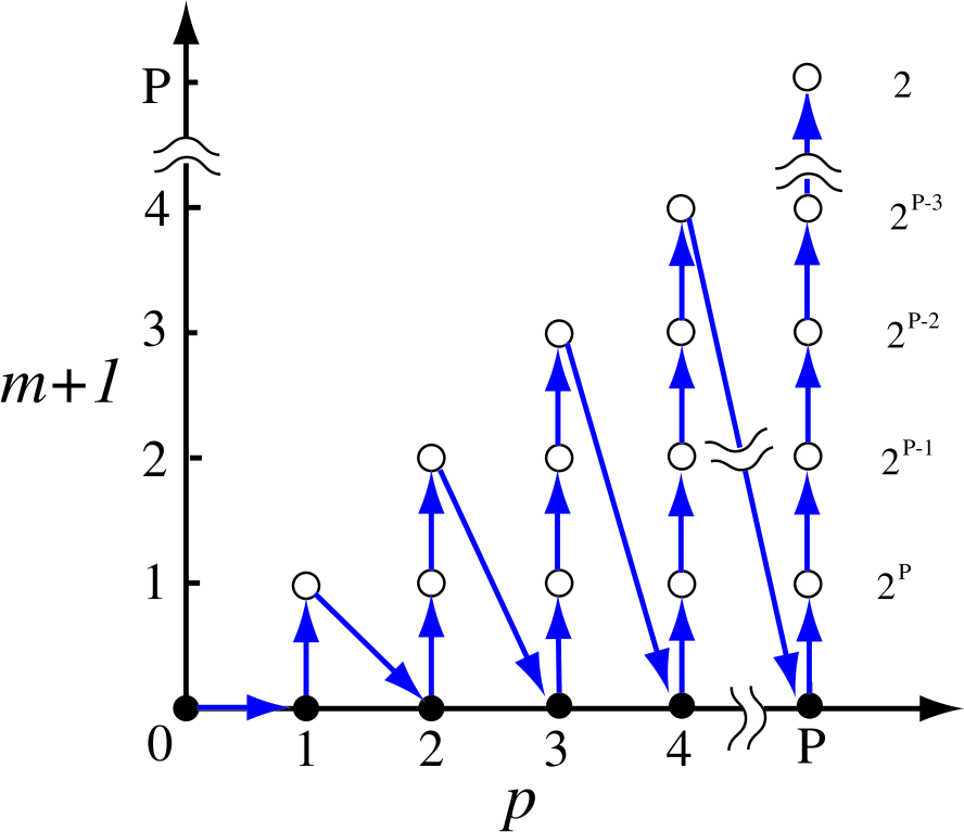
Figure 3: (Color online) The development of recurrence formulas Eqs. (28)-(32), which implies that the recurrence starts from $p=m+1=0$ and ends at $p=m+1=P$. The number in the right hand side is the multiplicity for similar calculations by Eq. (29) due to the index $n$ at each $m+1$.

We are now ready to calculate the selected elements of the Green function using the inverses of the Schur complements $S$ and $L$ calculated by the recurrence formulas of Eqs. (28)-(32). By noting that Eq. (21) has a recursive structure and the matrix $X$ is structured by the nested dissection, one can derive the following recurrence formula:

$X_{p+1,n}^{-1}$ $=$ (38)

where

$Y_{p,2n}^T$ $=$ $L_{p,2n}^T{S}_{p,n}^{-1},$

$Y_{p,2n+1}^T$ $=$ $L_{p,2n+1}^T{S}_{p,n}^{-1}.$ (39)

The recurrence formula Eq. (38) starts with $X_{0,n}^{-1}={(A_{0,n})}^{-1}$, adds contributions at $m+1=p$ for every $p$, and at last yields the inverse of the matrix $X$ as $X^{-1}=G(Z)=X_{P+1,0}^{-1}$. Since the calculation of each element for the inverse of $X$ can be independently performed, only the selected elements can be computed without calculating all the elements. The selected elements to be calculated are elements in the block matrices $A$, $B$, and $C$, each of which corresponds to a non-zero overlap matrix as discussed before. Thus, we can easily compute only the selected elements using a table function which stores the position for the non-zero elements in the block matrices $A$, $B$, and $C$.

A simple but nontrivial example is given in Appendix A to illustrate how the inverse of matrix is computed by the recurrence formulas, and also a similar way is presented to calculate a few eigenstates around a selected energy in Appendix B, while the proposed method can calculate the total energy of system without calculating the eigenstates.

2.3.3 Finding chemical potential

As well as the conventional DFT calculations, in the proposed method the chemical potential has to be adjusted so that the number of electrons can be conserved. However, there is no simpler way to know the number of electrons under a certain chemical potential before the contour integration by Eq. (8) with the chemical potential. Thus, we search the chemical potential by iterative methods for the charge conservation. Since the contour integration is the time-consuming step in the method, a smaller number of the iterative step directly leads to the faster calculation. Therefore, we develop a careful combination of several iterative methods to minimize the number of the iterative step for sufficient convergence. In general, the procedure for searching the chemical potential can be performed by a sequence (1)-(2) or (5)-(1)-(3)-(1)-(4)-(1)-(4)-(1)$\mathrm{\cdots }$ in terms of the following procedures. As shown later, the procedure enables us to obtain the chemical potential conserving the number of electrons within ${10}^{-8}$ electron/system by less than 5 iterations on an average.

(1) Calculation of the difference $\mathrm{\Delta }\mathit{}{N}_i$ in the total number of electrons. The difference $\mathrm{\Delta }{N}_i$ in the total number of electrons is defined with $\rho ({\mu }_i)$ calculated using Eq. (8) at a chemical potential ${\mu }_i$ by

$\mathrm{\Delta }{N}_i=\mathrm{Tr}\left(\rho ({\mu }_i)S\right)-N_{\mathrm{ideal}},$ (40)

where $N_{\mathrm{ideal}}$ is the number of electrons that the system should possess for the charge conservation. If $\mathrm{\Delta }{N}_i$ is zero, the chemical potential ${\mu }_i$ is the desired one of the system.

(2) Using the retarded Green function. If the difference $\mathrm{\Delta }{N}_i$ is large enough so that the interpolation schemes (3) and (4) can fail to guess a good chemical potential, the next trial chemical potential is estimated by using the retarded Green function. When the chemical potential of ${\mu }_{\mathrm{tri}}$ is considered, the correction $\delta N_{\mathrm{tri}}$ estimated by the retarded Green function to $\mathrm{\Delta }{N}_i$ is given by

$\delta N_{\mathrm{tri}}={\displaystyle {\int }_{E_{\min }}^{E_{\max }}}𝑑E\delta \rho (E)\mathrm{\Delta }f(E,{\mu }_{\mathrm{tri}}),$ (41)

where $\delta \rho (E)$ and $\mathrm{\Delta }f(E,{\mu }_{\mathrm{tri}})$ are defined by

$\delta \rho (E)=-{\displaystyle \frac{2}{\pi }}\mathrm{ImTr}\left(G(E+i\eta )S\right)$ (42)

with a small number $\eta$ (0.01 eV in this study) and

$\mathrm{\Delta }f(E,{\mu }_{\mathrm{tri}})$ $=$ $f\left({\displaystyle \frac{E-{\mu }_{\mathrm{tri}}}{k_{\mathrm{B}}T}}\right)-f\left({\displaystyle \frac{E-{\mu }_i}{k_{\mathrm{B}}T}}\right).$ (43)

The integration in Eq. (41) is numerically evaluated by a simple quadrature scheme such as trapezoidal rule with a similar number of points as for that of poles in Eq. (8), and the integration range can be determined by considering the surviving range of $\mathrm{\Delta }f(E,{\mu }_{\mathrm{tri}})$. The search of ${\mu }_{\mathrm{tri}}$ is performed by a bisection method until $\mathrm{\Delta }{N}_{\mathrm{cri}}>(\mathrm{\Delta }{N}_i+\delta N_{\mathrm{tri}})$, where $\mathrm{\Delta }{N}_{\mathrm{cri}}$ is a criterion for the convergence, and ${10}^{-8}$ electron/system is used in this study. It should be noted that the evaluation of Green function being the time-consuming part can be performed before the bisection method and a set of $\delta \rho (E)$ is stored for computational efficiency.

(3) Linear interpolation/extrapolation. In searching the chemical potential $\mu$, if two previous results (${\mu }_i,\mathrm{\Delta }{N}_i$) and (${\mu }_j,\mathrm{\Delta }{N}_j$) are available, a trial chemical potential ${\mu }_{\mathrm{tri}}$ is estimated by a linear interpolation/extrapolation method as:

${\mu }_{\mathrm{tri}}={\displaystyle \frac{{\mu }_j\mathrm{\Delta }{N}_i-{\mu }_i\mathrm{\Delta }{N}_j}{{\mu }_i-{\mu }_j}}.$ (44)

(4) Muller method[55, 56]. In searching the chemical potential $\mu$, if tree previous results (${\mu }_i,\mathrm{\Delta }{N}_i$), (${\mu }_j,\mathrm{\Delta }{N}_j$), and (${\mu }_k,\mathrm{\Delta }{N}_k$) are available, they can be fitted to a quadratic equation:

$\mathrm{\Delta }N=a{\mu }^2+b\mu +c,$ (45)

where $a$, $b$, and $c$ are found by solving a simultaneous linear equation of $3\times 3$ in size.[57] Then, ${\mu }_{\mathrm{tri}}$ giving $\mathrm{\Delta }N=0$ is a solution of Eq. (45), and given by

(46)

The selection of sign is unique because of the condition that the gradient at the solution must be positive, and the branching is taken into account to avoid the round-off error. As the iteration proceeds in search of the chemical potential, we have a situation that the number of available previous results is more than three. For the case, it is important to select three chemical potentials having smaller $\mathrm{\Delta }N$ and the different sign of $\mathrm{\Delta }N$ among three chemical potentials, since the guess of ${\mu }_{\mathrm{tri}}$ can be performed as the interpolation rather than the extrapolation.

(5) Extrapolation of chemical potential for the second step. During the self-consistent field (SCF) iteration, the chemical potential obtained at the last SCF step is used as the initial guess ${\mu }_1$ in the current SCF step. In addition, we estimate the second trial chemical potential by fitting a set of results $({\mu }_1^{(i)},\mathrm{\Delta }{N}_1^{(i)},{\mu }_2^{(i)},\mathrm{\Delta }{N}_2^{(i)})$, $({\mu }_1^{(j)},\mathrm{\Delta }{N}_1^{(j)},{\mu }_2^{(j)},\mathrm{\Delta }{N}_2^{(j)})$, and $({\mu }_1^{(k)},\mathrm{\Delta }{N}_1^{(k)},{\mu }_2^{(k)},\mathrm{\Delta }{N}_2^{(k)})$, where the subscript and the superscript in ${\mu }_0^{(i)}$ and $\mathrm{\Delta }{N}_0^{(i)}$ mean the iteration step in search of the chemical potential and the SCF step, respectively, at three previous SCF steps to the following equation:

$\mathrm{\Delta }{N}_2=a_1\mathrm{\Delta }{N}_1+a_2({\mu }_2-{\mu }_1)+a_3\mathrm{\Delta }{N}_1({\mu }_2-{\mu }_1),$ (47)

where $a_1$, $a_2$, and $a_3$ are found by solving a simultaneous linear equation of $3\times 3$ in size. Then, the chemical potential ${\mu }_2$ giving $\mathrm{\Delta }{N}_2=0$ can be estimated by solving Eq. (47) with respect to ${\mu }_2$ as follows:

${\mu }_{\mathrm{tri}}\equiv {\mu }_2={\mu }_1-{\displaystyle \frac{a_1\mathrm{\Delta }{N}_1}{a_2+a_3\mathrm{\Delta }{N}_1}}.$ (48)

It is found from numerical calculations that Eq. (48) provides a very accurate guess in most cases as the SCF calculation converges.

2.4 Computational complexity

We analyze the computational complexity of the proposed method. As discussed in the subsection Contour integration of the Green function, the number of poles for the contour integration is independent of the size of system. Thus, we focus on the computational complexity of the calculation of the Green function. For simplicity of the analysis we consider a finite chain, a finite square lattice, and a finite cubic lattice as representatives of 1D, 2D, and 3D systems, respectively, which are described by the $s$-valent NNTB models as in the explanation of the nested dissection. Note that the results in the analysis might be valid for more general cases with periodic boundary conditions. Since the computational cost is governed by Eq. (29), let us first analyze the computational cost of Eq. (29), while those of the other equations will be discussed later. Considering that the recurrence formula of Eq. (29) develops as shown in Fig. 3, and that the calculation of Eq. (29) corresponds to the open circle in the figure, the computational cost $t$ can be estimated by

$t\propto {\displaystyle \sum _{p=1}^P}{\displaystyle \sum _{m=0}^{p-1}}{\displaystyle \sum _{n=0}^{2^{P-m}-1}}{N}_m^{(1)}{N}_m^{(2)}{N}_p^{(3)},$ (49)

where $N_m^{(1)}$ and $N_m^{(2)}$ are the dimension of row and column in the matrix:

$\left(\begin{array}{c}\hfill L_{m,2n}^T\hfill \\ \hfill L_{m,2n+1}^T\hfill \\ \hfill -I\hfill \end{array}\right),$

and $N_p^{(3)}$ is the dimension of column in the matrix $Q_{p,m+1,n}^T$. Since Eq. (29) consists of a matrix product, the computational cost is simply given by $N_m^{(1)}{N}_m^{(2)}{N}_p^{(3)}$. Also it is noted that $N_m^{(1)}$ and $N_m^{(2)}$ depend on only $m$, and $N_p^{(3)}$ has dependency on only $p$ because of the simplicity of the systems we consider.

For the finite 1D chain system, we see that $N_m^{(1)}=N/(2^{P-m})$ and $N_m^{(2)}=N_p^{(2)}=1$ as listed in Table 1. Thus, the computational cost $t_{1\mathrm{D}}$ for the 1D system is estimated as

$t_{1\mathrm{D}}$ $\propto$ ${\displaystyle \sum _{p=1}^P}{\displaystyle \sum _{m=0}^{p-1}}{\displaystyle \sum _{n=0}^{2^{P-m}-1}}{\displaystyle \frac{N}{2^{P-m}}}$ (50)

$=$ ${\displaystyle \frac{1}{2}}NP(P+1).$

Noting $N\propto 2^P$, we see that the computational cost for the 1D system scales as O$(N{({\log }_2(N))}^2)$.

Table 1: Some of $N_m^{(2)}$ and $N_p^{(3)}$ in Eq. (49) for a finite 1D chain, a finite 2D square lattice, and a finite 3D cubic lattice described by the $s$-valent NNTB model. They depends on $m$ or $p$ for the 2D and 3D systems in a rather complicated way, while $N_{p,m,n}^{(1)}=\frac{N}{2^{P-m}}$ for all the cases. The unit for each case is given in parenthesis.

m+1 or p	P	P-1	P-2	P-3	P-4	P-5	P-6	P-7	P-8	P-9	P-10
1D (1)	1	1	1	1	1	1	1	1	1	1	1
2D ($N^{1/2}$)	1	$\frac{1}{2}$	$\frac{1}{2}$	$\frac{1}{4}$	$\frac{1}{4}$	$\frac{1}{8}$	$\frac{1}{8}$	$\frac{1}{16}$	$\frac{1}{16}$	$\frac{1}{32}$	$\frac{1}{32}$
3D ($N^{2/3}$)	1	$\frac{1}{2}$	$\frac{1}{4}$	$\frac{1}{4}$	$\frac{1}{8}$	$\frac{1}{16}$	$\frac{1}{16}$	$\frac{1}{32}$	$\frac{1}{64}$	$\frac{1}{64}$	$\frac{1}{128}$

For the finite 2D square lattice system, we see $N_m^{(1)}=N/(2^{P-m})$, and $N_m^{(2)}$ and $N_p^{(3)}$ depend on $m$ and $p$, respectively as shown in Table 1. To estimate the order of the computational cost we approximate $N_m^{(2)}$ and $N_p^{(3)}$ as $N_m^{(2)}\approx N^{1/2}/2^{\frac{1}{2}(P-m-1)}$ and $N_p^{(3)}\approx N^{1/2}/2^{\frac{1}{2}(P-p)}$ which are equal to or more than the corresponding exact number. Then, the computational cost $t_{2\mathrm{D}}$ for the 2D system can be estimated as follows:

$t_{2\mathrm{D}}$ $\propto$ ${\displaystyle \sum _{p=1}^P}{\displaystyle \sum _{m=0}^{p-1}}{\displaystyle \sum _{n=0}^{2^{P-m}-1}}{\displaystyle \frac{N}{2^{P-m}}}{N}_{p,m,n}^{(2)}{N}_{p,m,n}^{(3)}$ (51)

${\displaystyle \sum _{p=1}^P}{\displaystyle \sum _{m=0}^{p-1}}{\displaystyle \sum _{n=0}^{2^{P-m}-1}}{\displaystyle \frac{N}{2^{P-m}}}{\displaystyle \frac{N^{1/2}}{2^{\frac{1}{2}(P-m-1)}}}{\displaystyle \frac{N^{1/2}}{2^{\frac{1}{2}(P-p)}}}$

$=$ ${\displaystyle \frac{2N^2}{{(\sqrt{2}-1)}^2}}\left(2-\sqrt{2}+{\displaystyle \frac{\sqrt{2}}{2^P}}-{\displaystyle \frac{1}{2^P}}-{\displaystyle \frac{1}{2^{P/2}}}\right).$

Since the first two terms in parenthesis of the last line are the leading term, we see that the computational cost for the 2D system scales as O$(N^2)$.

For the finite 3D cubic lattice system we have $N_m^{(1)}=N/(2^{P-m})$ as well as the 1D and 2D systems. As shown in the analysis of the 2D systems, by approximating $N_m^{(2)}$ and $N_p^{(3)}$ as $N_m^{(2)}\approx N^{2/3}/2^{\frac{2}{3}(P-m-1)}$ and $N_p^{(3)}\approx N^{2/3}/2^{\frac{2}{3}(P-p)}$, which are equal to or more than the corresponding exact number, we can estimate the computational cost $t_{3\mathrm{D}}$ for the 3D system as follows:

$t_{3\mathrm{D}}$ $\propto$ ${\displaystyle \sum _{p=1}^P}{\displaystyle \sum _{m=0}^{p-1}}{\displaystyle \sum _{n=0}^{2^{P-m}-1}}{\displaystyle \frac{N}{2^{P-m}}}{N}_{p,m,n}^{(2)}{N}_{p,m,n}^{(3)}$ (52)

${\displaystyle \sum _{p=1}^P}{\displaystyle \sum _{m=0}^{p-1}}{\displaystyle \sum _{n=0}^{2^{P-m}-1}}{\displaystyle \frac{N}{2^{P-m}}}{\displaystyle \frac{N^{2/3}}{2^{\frac{2}{3}(P-m-1)}}}{\displaystyle \frac{N^{2/3}}{2^{\frac{2}{3}(P-p)}}}$

$=$ ${\displaystyle \frac{4N^{7/3}}{2^{2/3}6-9}}\left(-1+2^{2/3}-{\displaystyle \frac{1}{2^{2/3}{2}^{4P/3}}}+{\displaystyle \frac{1}{2^{2/3}{2}^{2P/3}}}-{\displaystyle \frac{2^{2/3}}{2^{2P/3}}}+{\displaystyle \frac{1}{2^{4P/3}}}\right).$

Since we see that the first two terms in parenthesis of the last line are the leading term, it is concluded that the computational cost for the 3D system scales as O$(N^{7/3})$.

We further analyze the computational cost of the other Eqs. (28), (30), (32), (38), and (39) which are the primary equations for the calculation of the Green function. Although the detailed derivations are not shown here, they can be derived in the same way as for Eq. (29). Table 2 shows the order of the computational cost for each equation. It is found that the computational cost is governed by Eq. (29), while the computational cost of Eq. (39) is similar to that of Eq. (29).

Table 2: Computational order of Eqs. (28), (29), (30), (32), (38), and (39), where the calculation of the inverse of the matrix $S$ is also included in estimating the computational cost of Eq. (32), and the sparse structure in the matrix $B$ is taken into account for Eqs. (28) and (32).

	1D	2D	3D
Eq. (28)	${({\log }_{2}N)}^2\mathit{\hspace{1em}}$	$N^{3/2}{\log }_{2}N\mathit{\hspace{1em}}$	$N^2\mathit{\hspace{1em}}$
Eq. (29)	$N{({\log }_{2}N)}^2$	$N^2$	$N^{7/3}$
Eq. (30)	$N{\log }_{2}N$	$N^{3/2}$	$N^{5/3}$
Eq. (32)	${\log }_{2}N$	$N$	$N^{4/3}$
Eq. (38)	$N$	$N^{3/2}$	$N^{5/3}$
Eq. (39)	$N{\log }_{2}N$	$N^2$	$N^{7/3}$

In addition to the analysis of the computational cost for the inverse calculations by Eq. (28)-(32), (38), and (39), we examine that for the nested dissection. The step (i) in the nested dissection involves a sorting procedure by the quicksort algorithm of which computational cost scales as $\frac{N}{2^p}{\log }_2\frac{N}{2^p}$ for a sequence with length of $\frac{N}{2^p}$, and thereby the computational cost for $d$-dimensional system can be estimated by

$d{\displaystyle \sum _{p=0}^P}\left({\displaystyle \frac{N}{2^p}}{\log }_2{\displaystyle \frac{N}{2^p}}\right)2^p={\displaystyle \frac{d}{2}}N{({\log }_{2}N)}^2.$ (53)

Also, considering that the steps (iii) and (iv) consist of search for the sequence with length of $\frac{N}{2^p}$, the the computational cost is found to be

$d{\displaystyle \sum _{p=0}^P}{\displaystyle \frac{N}{2^p}}{2}^p=dN{\log }_{2}N.$ (54)

The analysis indicates that the computational cost for the nested dissection scales as O$(N{({\log }_{2}N)}^2)$ for systems with any dimensionality. Thus, it is concluded that as a whole the proposed method scales as O$(N{({\log }_{2}N)}^2)$, O$(N^2)$, and O$(N^{7/3})$ for 1D, 2D, and 3D systems, respectively.[58]

3 NUMERICAL RESULTS

In the section several numerical calculations for the $s$-valent NNTB model and DFT are presented to illustrate practical aspects of the low-order scaling method. All the DFT calculations in this study were performed by the DFT code OpenMX.[59] The PAO basis functions[46] used in the DFT calculations are specified by H4.5-$s1$, C5.0-$s1p1$, N4.5-$s1p1$, O4.5-$s1p1$, and P6.0-$s1p1d1$ for deoxyribonuleic acid (DNA), C4.0-$s1p1$ for a single C${}_{60}$ molecule, and Pt7.0-$s2p2d1$ for a single Pt${}_{63}$ cluster, respectively, where the abbreviation of basis function such as C5.0-$s1p1$ represents that C stands for the atomic symbol, 5.0 the cutoff radius (bohr) in the generation by the confinement scheme, $s1p1$ means the employment of one primitive orbitals for each of $s$ and $p$ orbitals.[46] Since the PAO basis functions are pseudo-atomic orbitals with different cutoff radii depending on atomic species, the resultant Hamiltonian and overlap matrices have a disordered sparse structure, reflecting the geometrical structure of the system. Norm-conserving pseudopotentials are used in a separable form with multiple projectors to replace the deep core potential into a shallow potential.[60] Also a local density approximation (LDA) to the exchange-correlation potential is employed.[38]

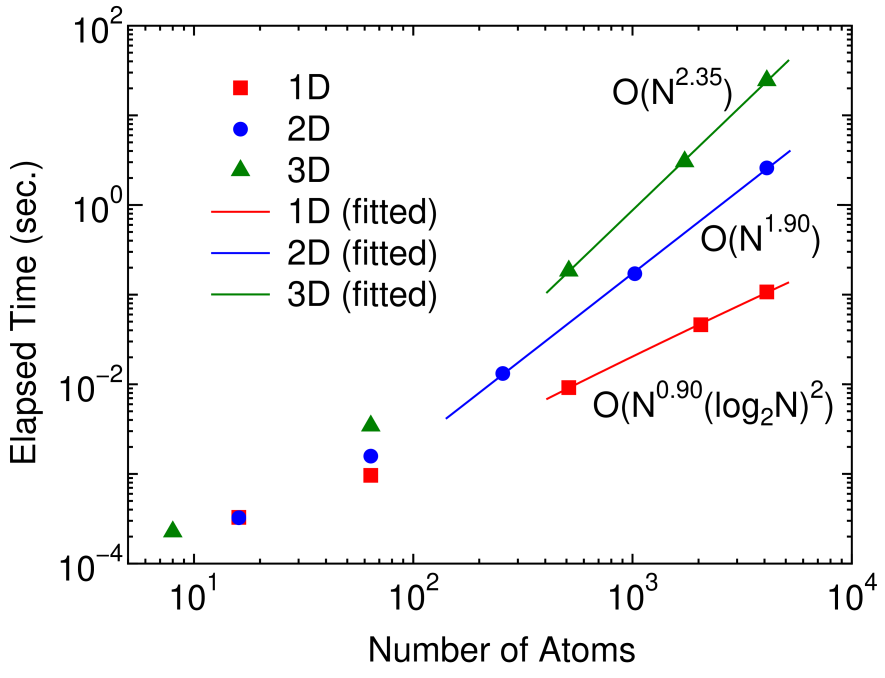
Figure 4: (Color online) The elapsed time of the inverse calculation by Eqs. (28)-(32) for a 1D linear chain, a 2D square lattice, and a 3D cubic lattice systems as a function of number of atoms in the unit cell under periodic boundary condition. The Hamiltonian of the systems are described by the $s$-valent NNTB models. The line for each system is obtained by a least square method, and the computational orders obtained from the fitted curves are O($N^{0.90}{({\log }_{2}N)}^2$), O($N^{1.90}$), and O($N^{2.35}$) for the 1D, 2D, and 3D systems, respectively. The size of domains at the innermost level is set to 20 for all the cases.

3.1 Scaling

As shown in the previous section, it is possible to reduce the computational cost from O($N^3$) to the low-order scaling without losing numerical accuracy. Here we validate the theoretical scaling property of the computational effort by numerical calculations. Figure 4 shows the elapsed time required for the calculation of inverse of a 1D linear chain, a 2D square lattice, and a 3D cubic lattice systems as a function of number of atoms in the unit cell under periodic boundary condition, which are described by the $s$-valent NNTB models. The last three points for each system are fitted to a function by a least square method, and the obtained scalings of the elapsed time are found to be O($N^{0.90}{({\log }_{2}N)}^2$), O($N^{1.90}$), and O($N^{2.35}$) for the 1D, 2D, and 3D systems, respectively. Thus, it is confirmed that the scaling of the computational cost is nearly the same as that of the theoretical estimation.

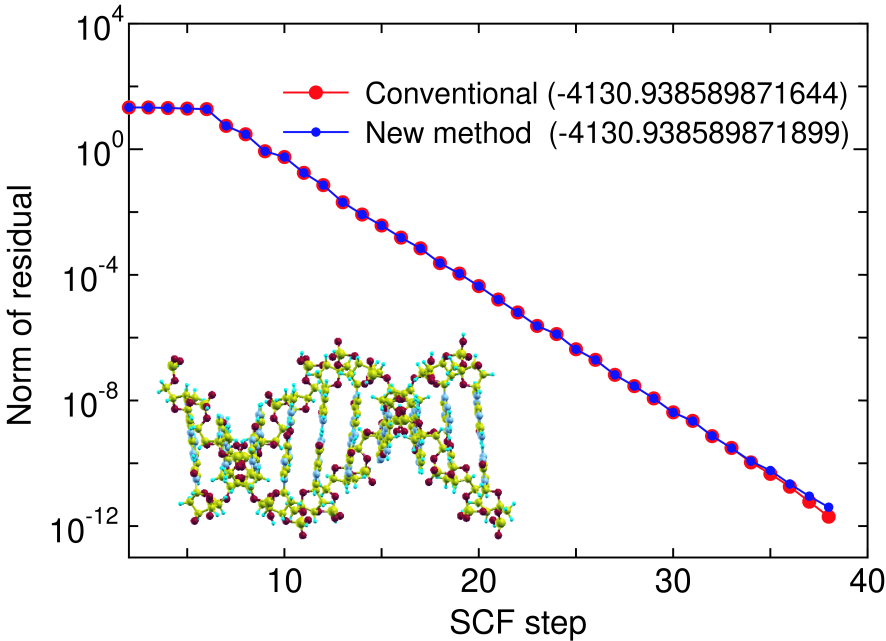
Figure 5: (Color online) The norm of residual in the SCF calculation of DNA, with a periodic double helix structure (650 atoms/unit) consisting of cytosines and guanines, calculated by the conventional and proposed methods, where the residual is defined as the difference between the input and output charge densities in momentum space. The electric temperature of 700 K and 80 poles for the contour integration are used. The number in parenthesis is the total energy (Hartree) of the system calculated by each method.

3.2 SCF calculation

To demonstrate that the proposed method is a numerically exact method even if the summation in Eq. (8) is terminated at a modest number of poles, we show the convergence in the SCF calculations calculated by the conventional diagonalization and the proposed methods for deoxyribonuleic acid (DNA) in Fig. 5, where 80 poles is used for the summation, and the electronic temperature is 700 K. It is clearly seen that the convergence property and the total energy are almost equivalent to those by the conventional method with only 80 poles. Table 3 also presents the rapid convergence of the total energy and forces in the SCF calculation as a function of the number of poles. In the case, the use of only 40 poles is enough to achieve the numerically exact results for not only the total energy but also the forces on atoms within numerical precision. Since the density matrix, total energy and forces on atoms can be very accurately evaluated within numerical precision as shown above, the low-order scaling method can be regarded as a variational method in practice.

Table 3: The absolute error of total energy $|E-E_{\mathrm{ref}}|$ (Hartree) and the mean absolute error (MAE) of forces on atoms (Hartree/bohr) in the SCF calculation of the same DNA system as for Fig. 5 as a function of the number of poles. The reference energy $E_{\mathrm{ref}}$ and forces are calculated by the conventional diagonalization method. The computational conditions are the same as for the calculations of Fig. 5.

Poles	$|E-E_{\mathrm{ref}}|$	MAE of forces
10	80.698617103348	0.040703500227
20	0.122135859603	0.000111580338
40	0.000000000162	0.000000000148
60	0.000000000264	0.000000000148
80	0.000000000255	0.000000000148
100	0.000000000251	0.000000000148

3.3 Iterative search of chemical potential

Although the computational cost of the proposed method can be reduced from the cubic to low-order scalings, the prefactor directly depends on the number of iterations in the iterative search of the chemical potential. To address how the combination of interpolation and extrapolation methods discussed before works to search a chemical potential which conserves the total number of electrons within a criterion, we show in Fig. 6 the number of iterations for finding the chemical potential, conserving the total number of electrons with a criterion of ${10}^{-8}$ electron/system, as a function of the SCF step for a C${}_{60}$ molecule, DNA, and a Pt${}_{63}$ cluster. Only few iterations are enough to achieve a sufficient convergence of the chemical potential as the SCF calculation converges, while a larger number of iterations are required at the initial stage of the SCF step. It turns out that the proper chemical potential can be searched by the mean iterations of 2.1, 2.4, and 4.0 for a C${}_{60}$ molecule, DNA, and a Pt${}_{63}$ cluster, respectively. The property of the iterative search is closely related to the energy gap of systems. The energy gap between the highest occupied and lowest unoccupied states of the C${}_{60}$ molecule, DNA, and Pt${}_{63}$ cluster are 1.95, 0.67, and 0.02 eV, respectively. For the C${}_{60}$ molecule and DNA with wide gaps the number of iterations for finding the chemical potential tends be large up to 10 SCF iterations, since the interpolation or extrapolation scheme may not work well due to the existence of the wide gap.

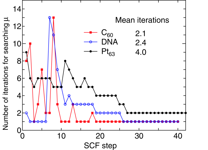
Figure 6: (Color online) The number of iterations for searching the chemical potential which conserves the total number of electrons within a criterion of ${10}^{-8}$ electron/system for a C${}_{60}$ molecule, DNA, and a Pt${}_{63}$ cluster, where the electric temperature of 600, 700, and 1000 K, and 80, 80, and 90 poles for the contour integration are used for the C${}_{60}$ molecule, DNA, and the Pt${}_{63}$ cluster,

However, once the charge density nearly converges, the approximate chemical potential in between the gap, which is the correct chemical potential at the previous SCF step, can satisfy the criterion of ${10}^{-8}$ electron/system. The situation does correspond to a small number of iterations after 10 SCF iterations. Even the trial chemical potential at the first step is the correct one within the criterion after 26 SCF iterations in these cases. For the Pt${}_{63}$ cluster with the narrow gap the number of iterations for finding the chemical potential is slightly lower than those of the a C${}_{60}$ molecule and DNA with the wide gaps at the initial stage of SCF iterations, which implies that the interpolation and extrapolation schemes by the procedures (3), (4), and (5) can give a good estimation of the chemical potential for the nearly continuous eigenvalue spectrum. In addition to this, one may find that in contrast to the cases with the wide gap, the correct chemical potential is found by two iterations as the charge density converges, since a little change of the chemical potential affects the distribution of charge density due to the narrow gap. However, the fact that only two iterations are sufficient even for the system with a narrow gap at the final stage of the SCF step suggests that the extrapolation by Eq. (48) works very well. Thus, we see from the numerical calculations that the correct chemical potential can be searched by only few iterations on an average with the combination of interpolation and extrapolation methods for systems with a wide variety of gap.

3.4 Parallel calculation

We demonstrate that the proposed method is suitable for the parallel computation because of the well separated data structure. It is apparent that the calculation of the Green function at each ${\alpha }_p$ in Eq. (8) can be independently performed without data communication among processors. Thus, we parallelize the summation in Eq. (8) by using the message passing interface (MPI) in which a nearly same number of poles are distributed to each process. The summation in Eq. (8) can be partly performed in each process, and the global summation is completed after all the calculations allocated to each process finish. In most cases the global summation can be a very small fraction of the computational time even including the MPI communication, since the amount of the data to be communicated is O($N$) due to the use of localized basis functions. In addition to the parallelization of the summation in Eq. (8), the calculation of the Green function can be parallelized in two respects. In the recursive calculations of Eqs. (28)-(32), one may notice that the calculation for different $n$ is independently performed, and also the calculations involving $V^T$ and $L^T$ in Eqs. (28)-(32) can be parallelized with respect to the column of $V^T$ and $L^T$ without communication until the recurrence calculations reach at $m+1=p$. For each $p$ the MPI communication only has to be performed at $m+1=p$. In our implementation only the latter part as for the calculation of the Green function is parallelized by a hybrid parallelization using MPI and OpenMP, which are used for internodes and intranode parallelization. As a whole, we parallelize the summation in Eq. (8) using MPI and the calculations involving $V^T$ and $L^T$ in Eqs. (28)-(32) using the hybrid scheme.

Figure 7 shows the speed-up ratio by the parallel calculation in the elapsed time of one SCF iteration. The speed-up ratio reaches about 350 and the elapsed time obtained is 3.76 $sec$ using 162 processes and 4 threads, which demonstrates the good scalability of the proposed method. On the other hand, the conventional diagonalization using Householder and QR methods scales up to only 21 processes, which leads to the speed-up ratio of about 10 and the elapsed time of 7.09 $sec$. Thus, we see that the proposed method is of great advantage to the parallel computation unlike the conventional method, while the comparison of the elapsed time suggests that the prefactor in the computational effort for the proposed method is larger than that of the conventional method.

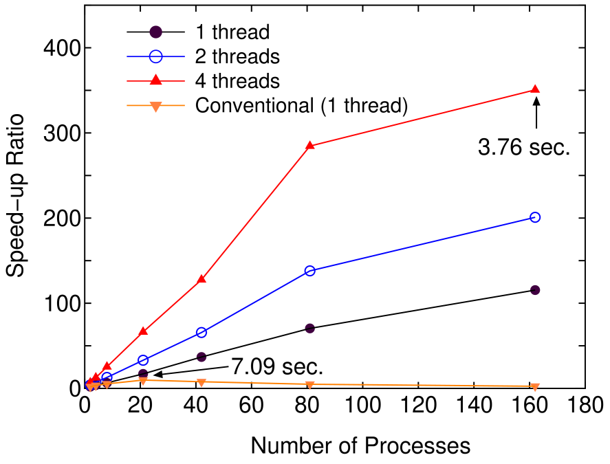
Figure 7: (Color online) Speed-up ratio in the parallel computation of the diagonalization in the SCF calculation for DNA by a hybrid scheme using MPI and OpenMP. The speed-up ratio is defined by $2T_2/T_p$, where $T_2$ and $T_p$ are the elapsed times obtained by two MPI processes and by the corresponding number of processes and threads. The structure of DNA is the same as in Fig. 5. The parallel calculations were performed on a Cray XT5 machine consisting of AMD opteron quad core processors (2.3 GHz). The electric temperature of 700 K and 80 poles for the contour integration are used. For comparison, the speed-up ratio for the parallel computation of the conventional scheme using Householder and QR methods is also shown for the case with a single thread.

4 CONCLUSIONS

An efficient low-order scaling method has been developed for large-scale DFT calculations using localized basis functions such as the PAO, FE, and wavelet basis functions, which can be applied to not only insulating but also metallic systems. The computational effort of the method scales as O($N{({\log }_{2}N)}^2$), O($N^2$), and O($N^{7/3}$) for 1D, 2D, and 3D systems, respectively. The method directly evaluates, based on two ideas, only selected elements in the density matrix which are required for the total energy calculation. The first idea is to introduce a contour integration method for the integration of the Green function in which the Fermi-Dirac function is expressed by a continued fraction. The contour integration enables us to obtain the numerically exact result for the integration within double precision at a modest number of poles, which allows us to regard the method as a numerically exact alternative to conventional O($N^3$) diagonalization methods. It is also shown that the number of poles needed for the convergence does not depend on the size of the system, but the spectrum radius of the system, which implies that the number of poles in the contour integration is unconcerned with the scaling property of the computation cost. The second idea is to employ a set of recurrence formulas for the calculation of the Green function. The set of recurrence formulas is derived from a recursive application of a block $LD{L}^T$ factorization using the Schur complement to a structured matrix obtained by a nested dissection for the sparse matrix $(ZS-H)$. The primary calculation in the recurrence formulas consists of matrix multiplications, and the computational scaling property is derived by the detailed analysis for the calculations. The chemical potential, conserving the total number of electrons, is determined by an iterative search which combines several interpolation and extrapolation methods. The iterative search permits to find the chemical potential by less than 5 iterations on an average for systems with a wide variety of gap. The good scalability in the parallel computation implies that the method is suitable for the massively parallel computation, and could extend the applicability of DFT calculations for large-scale systems together with the low-order scaling. It is also anticipated that the numerically exact method provides a platform in developing novel approximate efficient methods.

ACKNOWLEDGMENT

The author was partly supported by the Fujitsu lab., the Nissan Motor Co., Ltd., Nippon Sheet Glass Co., Ltd., and the Next Generation Super Computing Project, Nanoscience Program, MEXT, Japan. The author would like to thank Dr. M. Toyoda for critical reading of the manuscript.

Appendix A: AN EXAMPLE OF THE INVERSE CALCULATION

Since the proposed method to calculate the inverse of matrix is largely different from conventional methods, we show a simple but nontrivial example to illustrate the calculation of the inverse by using the set of recurrence formulas Eq. (28)-(32), (38), and (39), which may be useful to understand how the calculation proceeds. We consider a finite chain molecule consisting of seven atoms described by the same $s$-valent NNTB model as in the subsection Nested dissection, where all the on-site energies and hopping integrals are assumed to be 1. After performing the nested dissection, we obtain the following structured matrix:

(55)

where the blank means a zero element. It can be seen that the structure is same as in Eq. (22), and the system is divided into four domains with $P=1$. Then, we start from Eqs. (30) with $p=0$,

$V_{0,0,0}^T$ $=$ ${(A_{0,0})}^{-1}{(B_{0,0}[B_{0,0}])}^T$ (56)

$=$ $1\times 1=1\equiv L_{0,0}^T,$

$V_{0,0,1}^T$ $=$ ${(A_{0,1})}^{-1}{(B_{0,1}[B_{0,1}])}^T$ (57)

$=$ $1\times 1=1\equiv L_{0,1}^T,$

$V_{0,0,2}^T$ $=$ ${(A_{0,2})}^{-1}{(B_{0,2}[B_{0,2}])}^T$ (58)

$=$ $1\times 1=1\equiv L_{0,2}^T,$

$V_{0,0,3}^T$ $=$ ${(A_{0,3})}^{-1}{(B_{0,3}[B_{0,3}])}^T$ (59)

$=$ $1\times 1=1\equiv L_{0,3}^T,$

and proceed to calculate Eq. (32),

$S_{0,0}$ $=$ $C_{0,0}-B_{0,0}{L}_{0,0}^T-B_{0,1}{L}_{0,1}^T$ (60)

$=$ $1-1\times 1-1\times 1=-1,$

$S_{0,1}$ $=$ $C_{0,1}-B_{0,2}{L}_{0,2}^T-B_{0,3}{L}_{0,3}^T$ (61)

$=$ $1-1\times 1-1\times 1=-1.$

$X_{1,0}^{-1}$ and $X_{1,1}^{-1}$ which are precursors of the inverse of $X$ can be calculated by Eq. (38) and (39) as

$X_{1,0}^{-1}$ $=$ (62)

$=$

$=$

where $*$ means that the corresponding element is not calculated, and remains unknown, since these elements are not referred for further calculations. The precursor of $X_{1,1}^{-1}$ is found to be same as $X_{1,0}$ due to the same inner structure. As the next step, we set $p$ to 1, and calculate Eq. (30),

$V_{1,0,0}^T$ $=$ ${(A_{0,0})}^{-1}{(B_{1,0}[B_{0,0}])}^T$ (63)

$=$ $1\times 0=0,$

$V_{1,0,1}^T$ $=$ ${(A_{0,1})}^{-1}{(B_{1,0}[B_{0,1}])}^T$ (64)

$=$ $1\times 1=1,$

$V_{1,0,2}^T$ $=$ ${(A_{0,2})}^{-1}{(B_{1,1}[B_{0,2}])}^T$ (65)

$=$ $1\times 1=1,$

$V_{1,0,3}^T$ $=$ ${(A_{0,3})}^{-1}{(B_{1,1}[B_{0,3}])}^T$ (66)

$=$ $1\times 0=0,$

Eq. (28),

$Q_{1,1,0}^T$ $=$ $S_{0,0}^{-1}\left(B_{0,0}{V}_{1,0,0}^T+B_{0,1}{V}_{1,0,1}^T-{(B_{1,0}[C_{0,0}])}^T\right)$ (67)

$=$ $(-1)(1\times 0+1\times 1-0)=-1,$

$Q_{1,1,1}^T$ $=$ $S_{0,1}^{-1}\left(B_{0,2}{V}_{1,0,2}^T+B_{0,3}{V}_{1,0,3}^T-{(B_{1,1}[C_{0,1}])}^T\right)$ (68)

$=$ $(-1)(1\times 1+1\times 0-0)=-1,$

Eqs. (29) and (31),

$V_{1,1,0}^T$ $=$ $\left(\begin{array}{c}\hfill V_{1,0,0}^T\hfill \\ \hfill V_{1,0,1}^T\hfill \\ \hfill 0\hfill \end{array}\right)+\left(\begin{array}{c}\hfill L_{0,0}^T\hfill \\ \hfill L_{0,1}^T\hfill \\ \hfill -1\hfill \end{array}\right)Q_{1,1,0}^T$ (69)

$=$ $\left(\begin{array}{c}\hfill 0\hfill \\ \hfill 1\hfill \\ \hfill 0\hfill \end{array}\right)+\left(\begin{array}{c}\hfill 1\hfill \\ \hfill 1\hfill \\ \hfill -1\hfill \end{array}\right)(-1)=\left(\begin{array}{c}\hfill -1\hfill \\ \hfill 0\hfill \\ \hfill 1\hfill \end{array}\right)\equiv L_{1,0}^T,$

$V_{1,1,1}^T$ $=$ $\left(\begin{array}{c}\hfill V_{1,0,2}^T\hfill \\ \hfill V_{1,0,3}^T\hfill \\ \hfill 0\hfill \end{array}\right)+\left(\begin{array}{c}\hfill L_{0,2}^T\hfill \\ \hfill L_{0,3}^T\hfill \\ \hfill -1\hfill \end{array}\right)Q_{1,1,1}^T$

$=$ $\left(\begin{array}{c}\hfill 1\hfill \\ \hfill 0\hfill \\ \hfill 0\hfill \end{array}\right)+\left(\begin{array}{c}\hfill 1\hfill \\ \hfill 1\hfill \\ \hfill -1\hfill \end{array}\right)(-1)=\left(\begin{array}{c}\hfill 0\hfill \\ \hfill -1\hfill \\ \hfill 1\hfill \end{array}\right)\equiv L_{1,1}^T,$

and Eq. (32),

$S_{1,0}$ $=$ $C_{1,0}-B_{1,0}{L}_{1,0}^T-B_{1,1}{L}_{1,1}^T$ (71)

$=$

Finally updating the precursors $X_{1,0}^{-1}$ and $X_{1,1}^{-1}$ of the inverse of the matrix $X$ using Eqs. (38) and (39) yields the inverse of $X$ as follows:

$X_{2,0}^{-1}$ $=$ (72)

$=$

$=$

The calculated elements in the inverse $X^{-1}$ are found to be consistent with those by conventional methods such as the LU method. It is also noted that one can easily obtain the corresponding elements in the inverse of the original matrix using a table function generated in the nested dissection which converts the row or column index of the structured matrix to the original one.

Appendix B: Calculation of selected eigenstates

In the appendix, it is shown that a few eigenstates around a selected energy $\xi$ can be obtained by a similar way with the same computational complexity as in the calculation for the density matrix, though the proposed method directly computes the density matrix without explicitly calculating the eigenvectors.

We compute the few eigenstates around $\xi$ using a block shift-invert iterative method in which the generalized eigenvalue problem of Eq. (2) is transformed as

${(H-\xi S)}^{-1}S{c}_{\nu }={\displaystyle \frac{1}{{\epsilon }_{\nu }-\xi }}{c}_{\nu }.$ (73)

Then, the following iterative procedure yields a set of eigenstates around $\xi$ as the convergent result.

${𝐛}_l$ $=$ ${(H-\xi S)}^{-1}S{𝐜}_l,$ (74)

$⟨{𝐛}_l|\widehat{H}|{𝐛}_l⟩{𝐜}_{l+1}$ $=$ $⟨{𝐛}_l|\widehat{S}|{𝐛}_l⟩{𝐜}_{l+1}{\underset{¯}{\epsilon }}_{l+1},$ (75)

where $l$ is the iterative step, $\underset{¯}{\epsilon }$ is a square matrix consisting of diagonal elements, and $𝐛$ and $𝐜$ are a set of vectors, where the number of vectors is that of the selected states. The matrix multiplication in Eq. (74) and the solution of the generalized eigenvalue problem for Eq. (75) are repeated until convergence, and the convergent $𝐜$ and the diagonal elements of $\underset{¯}{\epsilon }$ correspond to the eigenstates around $\xi$. If the number of selected eigenstates is independent of the size of system, the computational cost required for Eq. (75) is O($N$), which arises from the matrix multiplications of $⟨{𝐛}_l|\widehat{H}|{𝐛}_l⟩$ and $⟨{𝐛}_l|\widehat{S}|{𝐛}_l⟩$. Therefore, the computational cost of the iterative calculation is governed by the matrix multiplication of ${(H-\xi S)}^{-1}{𝐲}_l^T$ in Eq. (74), where ${𝐲}_l^T=S{𝐜}_l$.

Here we show that the matrix multiplication of ${(H-\xi S)}^{-1}{𝐲}_l^T$ can be performed by a similar way with the same computational complexity as in the calculation for the density matrix. As an example of $(H-\xi S)$, let us consider the matrix $X$ given by Eq. (22). After the recurrence calculation of Eqs. (28)-(32), it turns out that the matrix $X$ is factorized as

$X=L_1{L}_{0}D{L}_0^T{L}_1^T$ (76)

with matrices defined by

and

where $I_{A_{0,0}}$ stands for an identity matrix with the same size as that of the matrix $A_{0,0}$, and the same rule applies to other cases. Then, we see that the inverse of $X$ is given by

$X^{-1}={(L_1^T)}^{-1}{(L_0^T)}^{-1}{D}^{-1}{(L_0)}^{-1}{(L_1)}^{-1}$ (77)

with matrices defined by

and

It should be noted that the inverses of $L_0$ and $L_1$ are remarkably simple, and that the inverse of $D$ is found to be a matrix consisting of diagonal block inverses. In general cases, we see that a matrix $X$ and its inverse are given by

$X=L_P\mathrm{\cdots }{L}_1{L}_{0}D{L}_0^T{L}_1^T\mathrm{\cdots }{L}_P^T,$ (78)

$X^{-1}$ $=$ ${(L_P^T)}^{-1}\mathrm{\cdots }{(L_1^T)}^{-1}{(L_0^T)}^{-1}{D}^{-1}$ (79)

$\times {(L_0)}^{-1}{(L_1)}^{-1}\mathrm{\cdots }{(L_P)}^{-1},$

where the inverse $L_p$ is given in a similar form as well as those of $L_0$ and $L_1$.

By considering Eq. (79) and the simple forms of ${(L_p)}^{-1}$, the matrix multiplication of $X^{-1}{𝐲}^T$ can be performed by the following three steps:

(i) The first step, ${({𝐲}^{\prime })}^T={(L_0)}^{-1}{(L_1)}^{-1}\mathrm{\cdots }{(L_P)}^{-1}{𝐲}^T$, is calculated by

${({𝐲}^{\prime }[I_{C_{p,n}}])}^T$ $=$ $-L_{p,2n}{(𝐲[L_{p,2n}])}^T-L_{p,2n+1}(𝐲{[L_{p,2n+1})}^T$ (80)

$+{(𝐲[I_{C_{p,n}}])}^T,$

${({𝐲}^{\prime }[I_{A_{0,n}}])}^T$ $=$ ${(𝐲[I_{A_{0,n}}])}^T,$ (81)

where $p=0,\mathrm{\cdots },P$ and $n=0,\mathrm{\cdots },2^{P-p}-1$ in Eq. (80), and $n=0,\mathrm{\cdots },2^P-1$ in Eq. (81).

(ii) The second step, ${({𝐲}^{\prime \prime })}^T=D^{-1}{({𝐲}^{\prime })}^T$, is calculated by

${({𝐲}^{\prime \prime }[I_{C_{p,n}}])}^T$ $=$ ${(S_{p,n})}^{-1}{({𝐲}^{\prime }[S_{p,n}])}^T,$ (82)

${({𝐲}^{\prime \prime }[I_{A_{0,n}}])}^T$ $=$ ${(A_{0,n})}^{-1}{({𝐲}^{\prime }[I_{A_{0,n}}])}^T,$ (83)

where $p=0,\mathrm{\cdots },P$ and $n=0,\mathrm{\cdots },2^{P-p}-1$ in Eq. (82), and $n=0,\mathrm{\cdots },2^P-1$ in Eq. (83).

(iii) The third step, ${(L_P^T)}^{-1}\mathrm{\cdots }{(L_1^T)}^{-1}{(L_0^T)}^{-1}{({𝐲}^{\prime \prime })}^T$, is performed by the following recurrence formulas:

${({𝐱}_{p+1}[L_{p,2n}])}^T$ $=$ ${({𝐱}_p[L_{p,2n}])}^T-{(L_{p,2n})}^T{({𝐱}_p[I_{C_{p,n}}])}^T,$ (84)

${({𝐱}_{p+1}[L_{p,2n+1}])}^T$ $=$ ${({𝐱}_p[L_{p,2n+1}])}^T$ (85)

$-{(L_{p,2n+1})}^T{({𝐱}_p[I_{C_{p,n}}])}^T,$

${({𝐱}_{p+1}[I_{C_{m,n}}])}^T$ $=$ ${({𝐱}_p[I_{C_{m,n}}])}^T,$ (86)

where ${𝐱}_0={𝐲}^{\prime \prime }$, $p+1=1,\mathrm{\cdots },P+1$, and $m=p,\mathrm{\cdots },P$. At the end of the recurrence calculation, we obtain the result of the multiplication as

$X^{-1}{𝐲}^T={𝐱}_{P+1}\equiv {(H-\xi S)}^{-1}{𝐲}^T.$ (87)

The computational effort of the three steps can be easily estimated by the same way as for the calculation of the inverse matrix, and summarized in Table 4. It is found that the the computational complexity of the three steps is lower than that of the calculation of the inverse matrix. Thus, if the number of selected eigenstates and the number of iterations for convergence are independent of the size of system, the computational effort of calculation of the selected eigenstates is governed by the recurrence calculation of Eqs. (28)-(32) even for the calculation of selected eigenstates. The scheme may be useful for calculation of eigenstates near the Fermi level.

Table 4: Computational order of Eqs. (80), (82), (83), (84), and (85).

	1D	2D	3D
Eq. (80)	$N{\log }_{2}N\mathit{\hspace{1em}}$	$N^{3/2}\mathit{\hspace{1em}}$	$N^{5/3}\mathit{\hspace{1em}}$
Eq. (82)	$N$	$N{\log }_{2}N$	$N^{4/3}$
Eq. (83)	$N$	$N$	$N$
Eqs. (84) +(85)	$N{\log }_{2}N$	$N^{3/2}$	$N^{5/3}$

References

- [1] P. Hohenberg and W. Kohn, Phys. Rev. 136, B864 (1964).
- [2] W. Kohn and L. J. Sham, Phys. Rev. 140, A1133 (1965).
- [3] R. Car and M. Parrinello, Phys. Rev. Lett. 55, 2471 (1985).
- [4] M.C. Payne, M.P. Teter, D.C. Allan, T.A. Arias, J.D. Joannopoulos, Rev. Mod. Phys. 64, 1045 (1992).
- [5] E.R. Davidson, in Methods in Computational Molecular Physics, Vol. 113 of NATO Advanced Study Institute, Series C: Mathematical and Physical Sciences, edited by G.H.F. Diercksen and S. Wilson (Plenum, New York, 1983), p. 95
- [6] P. Pulay, Chem. Phys. Lett. 73, 393 (1980).
- [7] D.M. Wood and A. Zunger, J. Phys. A 18, 1343 (1985).
- [8] M.P. Teter, M.C. Payne and D.C. Allan, Phys. Rev. B 40, 12255 (1989).
- [9] I. Stich, R. Car, M. Parrinello, and S. Baroni, Phys. Rev. B 39, 4997 (1989).
- [10] G. Kresse and J. Furthmuller, Phys. Rev. B 54, 11169 (1996).
- [11] A.S. Householder, J. ACM 5, 339 (1958).
- [12] G.H. Golub and C.F. van Loan, ”Matrix computations”, Johns Hopkins Univ Press (1996).
- [13] S. Goedecker, Rev. Mod. Phys. 71, 1085 (1999) and references therein.
- [14] S. Goedecker and G.E. Scuseria, Comp. Sci. Eng. 5, 14 (2003).
- [15] W. Yang, Phys. Rev. Lett. 66, 1438 (1991);
- [16] D.G. Pettifor, Phys. Rev. Lett. 63, 2480 (1989).
- [17] M. Aoki, Phys. Rev. Lett. 71, 3842 (1993).
- [18] T. Ozaki and K. Terakura, Phys. Rev. B 64, 195126 (2001).
- [19] T. Ozaki, Phys. Rev. B 74, 245101 (2006).
- [20] P. Ordejon, D.A. Drabold, M.P. Grumbach, and R.M. Martin, Phys. Rev. B 48, 14646 (1993); P. Ordejon, D.A. Drabold, R.M. Martin, and M.P. Grumbach, ibid. 51, 1456 (1995).
- [21] X.-P. Li, R.W. Nunes, and D. Vanderbilt, Phys. Rev. B 47, 10891 (1993).
- [22] D.R. Bowler and T. Miyazaki, J. Phys.: Condens. Matter 22, 074207 (2010).
- [23] N. D. M. Hine, P. D. Haynes, A. A. Mostofi, C.-K. Skylaris and M. C. Payne, Comput. Phys. Commun. 180, 1041 (2009).
- [24] K. Varga, Phys. Rev. B 81, 045109 (2010).
- [25] E. Tsuchida, J. Phys. Soc. Jpn. 76, 034708 (2007).
- [26] F. Shimojo, R.K. Kalia, A. Nakano, and P.Vashishta, Phys. Rev. B 77, 085103 (2008).
- [27] R. Takayama, T. Hoshi, T. Sogabe, S.-L. Zhang, T. Fujiwara, Phys. Rev. B 73, 165108 (2006).
- [28] M. Ogura and H. Akai, J. Comp. and Theo. Nanoscience 6, 2483 (2009).
- [29] R. Baer and M. Head-Gordon, Phys. Rev. B 58, 15296 (1998).
- [30] A.D. Daniels and G.E. Scuseria, J. Chem. Phys. 110, 1321 (1999).
- [31] K. Kitaura, E. Ikeo, T. Asada, T. Nakano, M. Uebayasi, Chem. Phys. Lett. 313, 701 (1999);
- [32] F.L. Gervasio, P. Carloni and M. Parrinello, Phys. Rev. Lett. 89 108102 (2002).
- [33] T. Miyazaki, D.R. Bowler, R. Choudhury, and M.J. Gillan, Phys. Rev. B 76, 115327 (2007); T. Miyazaki, D.R. Bowler, M.J. Gillan, and T. Ohno, J. Phys. Soc. Jpn. 77, 123706 (2008).
- [34] K. Nishio, T. Ozaki, T. Morishita, and M. Mikami, Phys. Rev. B 77, 201401(R) (2008); K. Nishio, T. Ozaki, T. Morishita, W. Shinoda, and M. Mikami, ibid. 77, 075431 (2008).
- [35] N. Zonias, P. Lagoudakis, and C.-K. Skylaris, J. Phys.: Condens. Matter 22, 025303 (2010).
- [36] J.I. Iwata, K. Shiraishi, and A. Oshiyama, Phys. Rev. B 77, 115208 (2008).
- [37] Y-K. Choe, E. Tsuchida, T. Ikeshoji, S. Yamakawa, and S. Hyodo, Phys. Chem. Chem. Phys. 11, 3892 (2009).
- [38] D.M. Ceperley and B.J. Alder, Phys. Rev. Lett. 45, 566 (1980); J.P. Perdew and A. Zunger, Phys. Rev. B 23, 5048 (1981).
- [39] J.P. Perdew, K. Burke, and M. Ernzerhof, Phys. Rev. Lett. 77, 3865 (1996).
- [40] L. Lin, J. Lu, L. Ying, R. Car, and Weinan E, Commun. Math. Sci. 7, 755 (2009).
- [41] S. Li, A. Ahmed, G. Klimeck, and E. Darve, J. Comp. Phys. 227, 9508 (2008).
- [42] D.E. Petersen, S. Li, K. Stokbro, H.H.B. Sorensen, P.C. Hansen, S. Skelboe, and E. Darve, J. Comp. Phys. 228, 5020 (2009).
- [43] K. Takahashi, J. Fagan, M.-S. Chin, in: 8th PICA Conference Proceedings, Minneapolis, Minn., 6369 (1973).
- [44] A.M. Erisman and W.F. Tinney, Numerical Mathematics 18, 177179 (1975).
- [45] Recently, Varga developed a similar method for quasi one-dimensional systems in which the density matrix is computed based on a contour integration and the evaluation of the Green function by making use of a factorization.[24] Although he suggested a possible way to extend his method to higher dimensional systems, the feasibility and the required computational cost remain unclear.
- [46] T. Ozaki, Phys. Rev. B. 67, 155108 (2003); T. Ozaki and H. Kino, ibid. 69, 195113 (2004);
- [47] E. Tsuchida and M. Tsukada, Phys. Rev. B 54, 7602 (1996).
- [48] L. Genovese, A. Neelov, S. Goedecker, T. Deutsch, S. A. Ghasemi, A. Willand, D. Caliste, O. Zilberberg, M. Rayson, A. Bergman, and R. Schneider, J. Chem. Phys. 129, 014109 (2008).
- [49] T. Ozaki, Phys. Rev. B 75, 035123 (2007).
- [50] When and , it can be shown that in Eq. (10) and , implying that they are not a large number, which is effective to avoid the numerical round-off error in the calculation of Eq. (10).
- [51] A. George, SIAM Journal on Numerical Analysis 10, 345363 (1973).
- [52] In a precise sense, we use domain to mean a system that we are now trying to bisect into two subdomains. In the recursive dissection, we obtain two subdomains after the dissection of the domain. Once we move to each subdomain to perform the next dissection, then the subdomain is called domain in the precise sense. In the text both the terms are distinguished for cases which may cause confusion.
- [53] G. Karypis and V. Kumar, SIAM Journal on Scientific Computing 20, 359 (1999).
- [54] T.A. Davis, SIAM, Philadelphia, Sept. 2006. Part of the SIAM Book Series on the Fundamentals of Algorithms.
- [55] D.E. Muller, Math. Tables Other Aids Comput. 10, 208215 (1956).
- [56] X. Wu, Appl. Math. Comput. 166, 299311 (2005).
- [57] Although the coefficients , , and can be analytically evaluated, the round-off error in the analytically evaluated solution is nonnegligible as converges to zero. In order to avoid the numerical problem, we refine , , and by minimizing a function with the analytically evaluated coefficients as initial values. We find that the coefficients refined by the minimization are much more accurate than the analytic ones for serious cases, and that the refinement is quite effective to avoid the numerical instability.
- [58] It is noted that the recurrence formula derived by Lin et al. allows us to compute selected elements in O operations for 3D systems,[40] which is superior to our recurrence formulas. However, the size of separators in their way for the nested dissection can be larger than that of our separators especially for the case that basis functions overlap with a number of other basis functions like in the PAO basis functions, which leads to a large prefactor for the computational cost in spite of the lower scaling. Also, the comparison with the algorithm by Takahashi et al.[43] and Erisman and Tinney[44] will be in a future work.
- [59] The code, OpenMX, pseudo-atomic basis functions, and pseudopotentials are available on a web site (http://www.openmx-square.org/).
- [60] N. Troullier and J.L. Martins, Phys. Rev. B 43, 1993 (1991).