Eigenchannel analysis

In the step 3, transmission eigenchannels are calculated optionally. Parameters for this calculation are as follows:

    NEGF.tran.Channel          on        #  default on
    NEGF.Channel.Nkpoint        1        # default=1
    <NEGF.Channel.kpoint
    0.0  0.0
    NEGF.Channel.kpoint>
    # default 0.0 0.0
    NEGF.Channel.Nenergy        1        # default=1
    <NEGF.Channel.energy
    0.0
    NEGF.Channel.energy>
    # default 0.0
    NEGF.Channel.Num    5    # defualt=5(for collinear), 10(for Non-collinear)

• NEGF.tran.Channel

  If NEGF.tran.Channel is set to on, the eigenchannel is calculated.

• NEGF.Channel.Nkpoint, <NEGF.Channel.kpoint, NEGF.Channel.kpoint>

  These keywords specify the k point, at which eigenchannels are calculated. Please write a ${\bf k}$ points per one line between <NEGF.Channel.kpointand NEGF.Channel.kpoint>; the total number of ${\bf k}$ is NEGF.Channel.Nkpoint. The coordinate of the $k$ is two dimensional fractional coordinate; ${\bf k}$ should be specified as coefficients of two reciprocal lattice vector perpendicular to the transmittion direction.

• NEGF.Channel.Nenergy, <NEGF.Channel.energy, NEGF.Channel.energy>

  These keywords specify the energy, at which eigenchannels are calculated. Please write a energy per one line between <NEGF.Channel.energy and NEGF.Channel.energy>; the total number of energies is NEGF.Channel.Nenergy. The unit should be [eV] and the energy should be measured from the electrochemical potential of the left lead.

• NEGF.Channel.Num

  It specifies the number of eigenchannels that are printed in the real space representation. In each ${\bf k}$, energy, spin, NEGF.Channel.Num eigenchannels in descending order about transmission eigenvalues are printed in the Gaussian cube format; the real and imaginary part is printed separately.

In the calculation of eigenchannels, openmx makes the following standard output:

**************************************************
 Calculation of transmission eigenchannels starts
**************************************************

  File index : negf-8zgnr-0.3.traneval#k_#E_#spin negf-8zgnr-0.3.tranevec#k_#E_#spin 

  myid0 =   0, #k :    0, N_{ort} / N_{nonort} : 380 / 380 
  PE    0 generates ./negf-8zgnr-0.3.traneval0_0_0 . Sum(eigenval) :   0.031643 
  PE    0 generates ./negf-8zgnr-0.3.traneval0_0_1 . Sum(eigenval) :   0.000508 

  Eigenchannel calculation finished 
  They are written in plottable files. 
  File index : negf-8zgnr-0.3.tranec#k_#E_#spin_#branch_r.cube(.bin)  
               negf-8zgnr-0.3.tranec#k_#E_#spin_#branch_i.cube(.bin)  

  ./negf-8zgnr-0.3.tranec0_0_0_0_r.cube     ./negf-8zgnr-0.3.tranec0_0_0_0_i.cube 
  ./negf-8zgnr-0.3.tranec0_0_0_1_r.cube     ./negf-8zgnr-0.3.tranec0_0_0_1_i.cube 
  ./negf-8zgnr-0.3.tranec0_0_0_2_r.cube     ./negf-8zgnr-0.3.tranec0_0_0_2_i.cube 
  ./negf-8zgnr-0.3.tranec0_0_0_3_r.cube     ./negf-8zgnr-0.3.tranec0_0_0_3_i.cube 
  ./negf-8zgnr-0.3.tranec0_0_0_4_r.cube     ./negf-8zgnr-0.3.tranec0_0_0_4_i.cube 
  ./negf-8zgnr-0.3.tranec0_0_1_0_r.cube     ./negf-8zgnr-0.3.tranec0_0_1_0_i.cube 
  ./negf-8zgnr-0.3.tranec0_0_1_1_r.cube     ./negf-8zgnr-0.3.tranec0_0_1_1_i.cube 
  ./negf-8zgnr-0.3.tranec0_0_1_2_r.cube     ./negf-8zgnr-0.3.tranec0_0_1_2_i.cube 
  ./negf-8zgnr-0.3.tranec0_0_1_3_r.cube     ./negf-8zgnr-0.3.tranec0_0_1_3_i.cube 
  ./negf-8zgnr-0.3.tranec0_0_1_4_r.cube     ./negf-8zgnr-0.3.tranec0_0_1_4_i.cube

In this case, 22 files, negf-8zgnr-0.3.treval0_0_0, negf-8zgnr-0.3.tranevec0_0_0,
negf-8zgnr-0.3.tranec0_0_0_0_r.cube - negf-8zgnr-0.3.tranec0_0_1_4_r.cube,
negf-8zgnr-0.3.tranec0_0_0_0_i.cube - negf-8zgnr-0.3.tranec0_0_1_4_i.cube, are generated.

• System.Name.traneval{#k}_{#E}_{#s}

  This file contains transmission eigenvalues of all eigenchannels in the {#k}th k, {#E}th energy, and {#s}th spin.

• System.Name.tranevec{#k}_{#E}_{#s}

  This file contains LCAO components of all eigenchannels in the {#k}th k, {#E}th energy, and {#s}th spin.

  e. g. / negf-chain.tranevec0_0_0

***********************************************************
***********************************************************
        Eigenvalues and LCAO coefficients                  
        at the k-points specified in the input file.       
***********************************************************
***********************************************************


   # of k-point = 0
   k2=   0.00000 k3=   0.00000

   # of Energy = 0
   e=   0.00000 

   Spin = Up 

   Real (Re) and imaginary (Im) parts of LCAO coefficients


                          1                   2                   3                   4              
                         0.9778              0.0000              0.0000              0.0000          

                          Re        Im        Re        Im        Re        Im        Re        Im   

   1   C 0 s            -0.00000  -0.00000  -0.00000   0.00000   0.00000   0.00000  -0.00000   0.00000
         1 s            -0.00000  -0.00000  -0.00000  -0.00000   0.00000  -0.00000   0.00000  -0.00000
         0 px           -0.63002  -1.49377  -0.14466   0.00019   0.01644  -0.00032  -0.07885   0.00095
         0 py            0.00000   0.00000   0.00000   0.00000  -0.00000   0.00000   0.00000   0.00000
         0 pz            0.00000  -0.00000   0.00000  -0.00000  -0.00000  -0.00000  -0.00000  -0.00000
   2   C 0 s            -0.00000  -0.00000  -0.00000  -0.00000   0.00000  -0.00000   0.00000  -0.00000
         1 s             0.00000   0.00000  -0.00000  -0.00000  -0.00000   0.00000  -0.00000   0.00000
         0 px            0.18040  -0.03816  -0.00452   0.00009  -0.00545  -0.00010  -0.01970  -0.00004
         0 py           -0.00000  -0.00000  -0.00000   0.00000   0.00000   0.00000   0.00000   0.00000
         0 pz            0.00000  -0.00000  -0.00000   0.00000  -0.00000  -0.00000  -0.00000  -0.00000
   3   C 0 s             0.00000   0.00000   0.00000  -0.00000  -0.00000   0.00000  -0.00000   0.00000
         1 s            -0.00000  -0.00000   0.00000   0.00000   0.00000  -0.00000   0.00000  -0.00000
         0 px            2.06634   0.40490   0.11067   0.00023  -0.06068   0.00009  -0.06690  -0.00042
         0 py            0.00000   0.00000   0.00000  -0.00000  -0.00000   0.00000  -0.00000   0.00000
         0 pz            0.00000   0.00000   0.00000   0.00000  -0.00000  -0.00000   0.00000  -0.00000
   4   C 0 s             0.00000   0.00000   0.00000   0.00000  -0.00000  -0.00000  -0.00000  -0.00000
         1 s            -0.00000  -0.00000  -0.00000  -0.00000  -0.00000   0.00000  -0.00000   0.00000

• System.Name.tranec{#k}_{#E}_{#s}_{#c}_r.cube,
  System.Name.tranec{#k}_{#E}_{#s}_{#c}_i.cube

  This file contains the real or the imaginary part of the eigenchannel in the Gaussian cube format. We can display isosurfaces from this files by using VESTA, XCrysDen, etc.

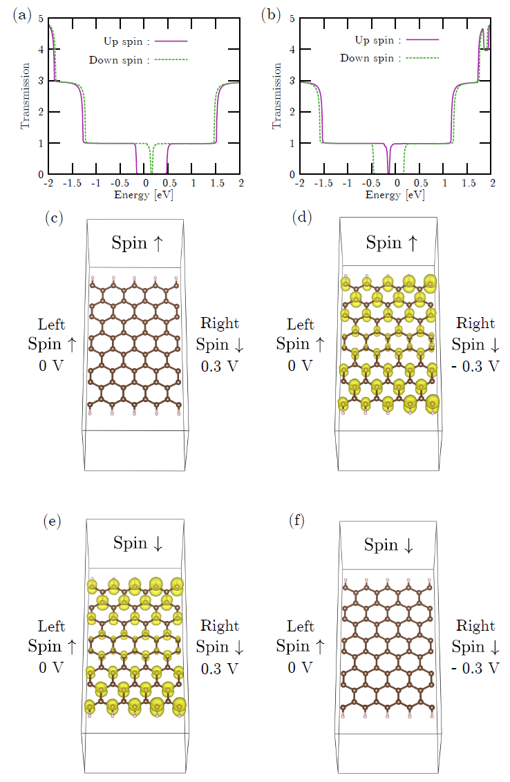
  For example, eigenchannels in 8-zigzag graphene nanoribbon with an antiferromagnetic junction under a finite bias voltage of 0.3 V is shown in Fig. 35.

Figure 35: (a) Spin dependent transmission under a bias voltage of 0.3 V, (b) Spin dependent transmission under a bias voltage of -0.3 V, (c) An eigenchannel at an energy of 0 eV, spin $\uparrow$, and 0.3 V as a bias voltage, (d) An eigenchannel at an energy of 0 eV, spin $\uparrow$, and - 0.3 V as a bias voltage, (e) An eigenchannel at an energy of 0 eV, spin $\downarrow$, and 0.3 V as a bias voltage, and (f) An eigenchannel at an energy of 0 eV, spin $\downarrow$, and - 0.3 V as a bias voltage in 8-zigzag graphene nanoribbon with an antiferromagnetic junction (The spin is $\uparrow$ in the left region and it is $\downarrow$ in the right region.) are depicted. The level of isosurfaces are identical in these figures; when the transmission is small, the eigenchannel itself is also small.