A simple way of performing large-scale calculations is firstly to employ
an O(![]() ) method to obtain a self-consistent charge density, and then
is to just once diagonalize using the conventional diagonalization method
under the self-consistent charge density to obtain full wave functions.
As an illustration of this procedure, we show a large-scale calculation of
a multiply connected carbon nanotube (MCCN) consisting of 564 carbon atoms.
First, the SCF calculation of a MCCN was performed using the O(
) method to obtain a self-consistent charge density, and then
is to just once diagonalize using the conventional diagonalization method
under the self-consistent charge density to obtain full wave functions.
As an illustration of this procedure, we show a large-scale calculation of
a multiply connected carbon nanotube (MCCN) consisting of 564 carbon atoms.
First, the SCF calculation of a MCCN was performed using the O(![]() ) DC method
and 32 processors of 2.4 GHz Opteron, where C4.5-s2p1 (basis function),
100 Ryd (scf.energycutoff), 1.0e-7 (scf.criterion),
6.5 Å (orderN.HoppingRanges), 2 (orderN.NumHoppings)
and RMM-DIISK (mixing scheme) were used. The input file is MCCN.dat
in the directory 'work'.
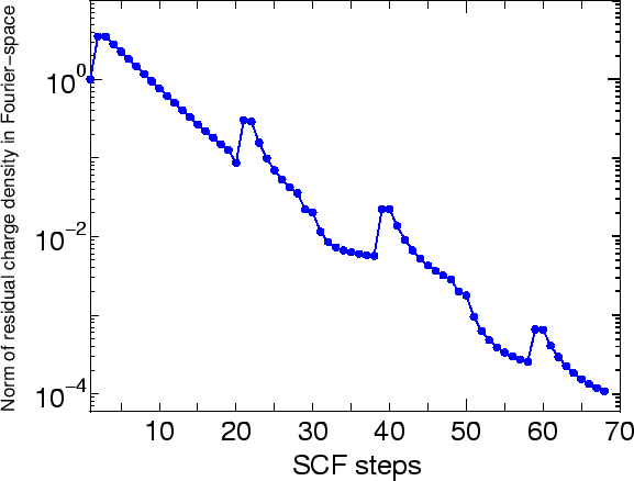
Figure 20 shows the norm of residual charge density in Fourier space as
a function of SCF steps. We see that 68 SCF steps is enough to
obtain a convergent charge density for this system, where the
computational time was 24 minutes.
) DC method
and 32 processors of 2.4 GHz Opteron, where C4.5-s2p1 (basis function),
100 Ryd (scf.energycutoff), 1.0e-7 (scf.criterion),
6.5 Å (orderN.HoppingRanges), 2 (orderN.NumHoppings)
and RMM-DIISK (mixing scheme) were used. The input file is MCCN.dat
in the directory 'work'.
Figure 20 shows the norm of residual charge density in Fourier space as
a function of SCF steps. We see that 68 SCF steps is enough to
obtain a convergent charge density for this system, where the
computational time was 24 minutes.
 |
Then, the following keywords were set in
    scf.maxIter                1
    scf.EigenvalueSolver    Band
    scf.Kgrid              1 1 1
    scf.restart               on
    MO.fileout                on
    num.HOMOs                  2
    num.LUMOs                  2
    MO.Nkpoint                 1
    <MO.kpoint
      0.0  0.0  0.0
    MO.kpoint>
And we calculated the same system in order to obtain wave functions
using 32 processors of 2.4 GHz Opteron, where the computational time
was 24 minutes.
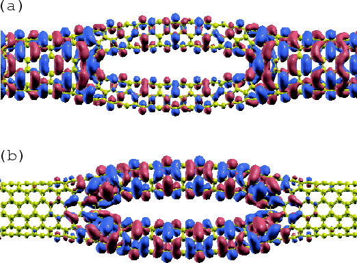
Figure 20 shows isosurface maps of the HOMO and LUMO (![]() -point)
of MCCN calculated by the above procedure.
Although the difference between the O(
-point)
of MCCN calculated by the above procedure.
Although the difference between the O(![]() ) method and the conventional
diagonalization scheme in the computational time is not significant in
this example, the procedure will be useful for larger system including
more than a thousand atoms.
) method and the conventional
diagonalization scheme in the computational time is not significant in
this example, the procedure will be useful for larger system including
more than a thousand atoms.
 |