Steepest decent optimization

An example of the geometry optimization is illustrated in this Section. As the initial structure, we considered the methane molecule given in the Section 'Input file', but the x-coordinate of the carbon atom of a methane molecule was moved to 0.3 Å as follows:

   <Atoms.SpeciesAndCoordinates
     1   C      0.300000    0.000000    0.000000     2.0  2.0 
     2   H     -0.889981   -0.629312    0.000000     0.5  0.5
     3   H      0.000000    0.629312   -0.889981     0.5  0.5
     4   H      0.000000    0.629312    0.889981     0.5  0.5
     5   H      0.889981   -0.629312    0.000000     0.5  0.5
   Atoms.SpeciesAndCoordinates>

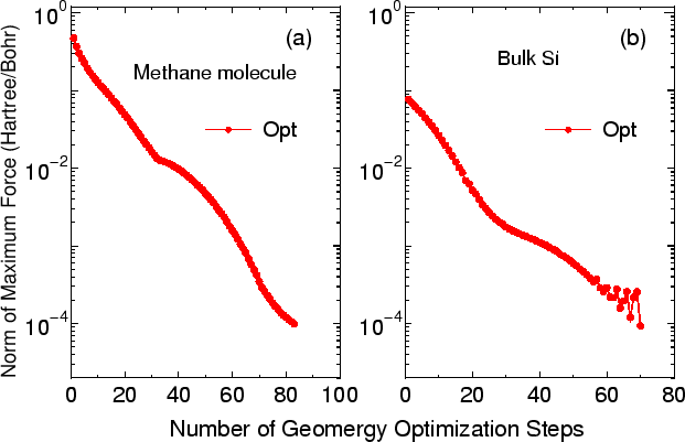
Then, a keyword 'MD.type' was specified as 'Opt', and set to 200 for a keyword 'MD.maxIter'. The 'Opt' is based on a simple steepest decent method with a variable prefactor. Figure 8 (a) shows the convergence history of the norm of the maximum force on atom as a function of the number of the optimization steps. We see that the norm of the maximum force on atom smoothly converges. Using Methane2.dat in the directory 'work', you can trace the calculation.

Figure: The norm of the maximum force on atom of (a) a methane molecule (b) silicon in the diamond structure as a function of the number of MD steps. The initial structures were ones distorted from the the equilibrium structures. The input files are Methane2.dat and Si8.dat in the directory 'work', respectively.