
Manual of OpenFFT Version 1.1 (PDF)
Installation
Requirements: OpenFFT requires FFTW3 (or FFTW3 wrappers such as those provided by the Intel MKL library), a C compiler, and an MPI library. Fortran users will also need a Fortran compiler to compile the Fortran sample programs.
Step 1: Download and install FFTW3. Assume that FFTW3 is installed in /opt/fftw3. Those who already have the Intel MKL library or FFTW3 wrappers installed can skip this step.
Step 2: Download and extract the OpenFFT tarball. Assume that OpenFFT is extracted to /opt/openfft1.1.Step 3:
Modify CC (the C compiler) and LIB (the library path
to FFTW3) in makefile in the root folder of
OpenFFT to reflect your
environment. Fortran users also need to specify FC (the
Fortran compiler)
to compile the sample programs. Samples of CC (and FC) and LIB in
several environments are given in
makefile.
CC = mpicc -O3
-I/opt/3/include -I./include

LIB = -L/opt/fftw3/lib -lfftw3

FC = mpif90 -O3
-I/opt/fftw3/include -I./include
Step 4:
Issue the make command to compile
and
install the OpenFFT
library. The library will be made available at
/opt/openfft1.1/lib/libopenfft.a if successful.
mpicc -O3 -o
userprogram
userprogram.c -I/opt/fftw3/include -I/opt/openfft1.1/include
-L/opt/fftw3/lib -lfftw3 -L/opt/openfft1.1/lib -lopenfft

mpif90 -O3 -o userprogram
userprogram.f90 -I/opt/fftw3/include -I/opt/openfft1.1/include
-L/opt/fftw3/lib -lfftw3 -L/opt/openfft1.1/lib -lopenfft
Directory Structure
toplevel: this is wheremakefileis located, as well asREADME.source: core source files of the package.openfft_init_c2c_3d.c: initialization of complex-to-complex transforms.openfft_init_r2c_3d.c: initialization of real-to-complex transforms.openfft_exec_c2c_3d.c: execution of complex-to-complex transforms.openfft_exec_r2c_3d.c: execution of real-to-complex transforms.openfft_finalize.c: finalization of transforms.openfft_dtime.c: built-in time measurement.include: C and Fortran header files.lib: the library file is installed here if successful.samples: sample programs for illustrating how to use OpenFFT.C: C sample programs.FORTRAN: Fortran sample program.sdoc: documents on the website of OpenFFT.
Sample Programs
- C sample programs:
check_c2c_3d.c: This program illustrates how to use the c2c interface. It can be executed with an arbitrary number of processes. Its input and output should match the corresponding values in check_c2c_3d.dat. This program does not require any input parameter.check_r2c_3d.c: This program illustrates how to use the r2c interface. It can be executed with an arbitrary number of processes. Its input and output should match the corresponding values in check_r2c_3d.dat. This program does not require any input parameter.timing_c2c_3d.c: This program is used for benchmarking performance of the c2c interface with timing and GFLOPS results. It can be executed with an arbitrary number of processes. Time is measured by MPI_Wtime(). A numeric input parameter can be provided for specifying the size of the 3 dimensions. If no input parameter is provided, it will be executed with a default size of 128^3 data points.timing_r2c_3d.c: This program is used for benchmarking performance of the r2c interface with timing and GFLOPS results. It can be executed with an arbitrary number of processes. Time is measured by MPI_Wtime(). A numeric input parameter can be provided for specifying the size of the 3 dimensions. If no input parameter is provided, it will be executed with a default size of 128^3 data points.breaktime_c2c_3d.c: This program is used for benchmarking performance of the c2c interface with timing result broken down into several parts and GFLOPS. It can be executed with an arbitrary number of processes. Time is measured by the built-in time measurement function. A numeric input parameter can be provided for specifying the size of the 3 dimensions. If no input parameter is provided, it will be executed with a default size of 128^3 data points. Please note that the timing breakdown can only be correctly done with the communication pattern number 6, as other patterns may feature communication and computation overlap.breaktime_r2c_3d.c: This program is used for benchmarking performance of the r2c interface with timing result broken down into several parts and GFLOPS. It can be executed with an arbitrary number of processes. Time is measured by the built-in time measurement function. A numeric input parameter can be provided for specifying the size of the 3 dimensions. If no input parameter is provided, it will be executed with a default size of 128^3 data points. Please note that the timing breakdown can only be correctly done with the communication pattern number 6, as other patterns may feature communication and computation overlap.- Fortran sample programs:
check_c2c_3d.f90: This program illustrates how to use the c2c interface. It can be executed with an arbitrary number of processes. Its input and output should match the corresponding values in check_c2c_3d.dat. This program does not require any input parameter.check_r2c_3d.f90: This program illustrates how to use the r2c interface. It can be executed with an arbitrary number of processes. Its input and output should match the corresponding values in check_r2c_3d.dat. This program does not require any input parameter.timing_c2c_3d.f90: This program is used for benchmarking performance of the c2c interface with timing and GFLOPS results. It can be executed with an arbitrary number of processes. Time is measured by MPI_Wtime(). A numeric input parameter can be provided for specifying the size of the 3 dimensions. If no input parameter is provided, it will be executed with a default size of 128^3 data points.timing_r2c_3d.f90: This program is used for benchmarking performance of the r2c interface with timing and GFLOPS results. It can be executed with an arbitrary number of processes. Time is measured by MPI_Wtime(). A numeric input parameter can be provided for specifying the size of the 3 dimensions. If no input parameter is provided, it will be executed with a default size of 128^3 data points.
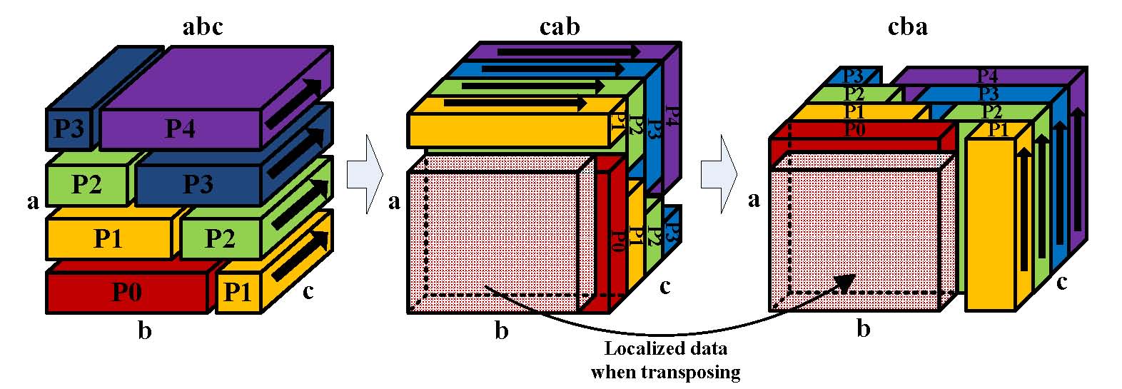
Domain Decomposition
Tuning of Communication
- 0: auto-tuning of communication, where OpenFFT automatically performs tests with all of the following patterns and picks the best performer in run time (recommended for high performance).
- 1: MPI_Alltoallv.
- 2: MPI_Isend and MPI_Irecv within sub-groups of 32 processes.
- 3: MPI_Isend and MPI_Irecv with communication-computation overlap.
- 4: MPI_Isend and MPI_Irecv within sub-groups of 32 processes with communication-computation overlap.
- 5: MPI_Sendrecv.
- 6: MPI_Isend and MPI_Irecv.
- Others: default communication, which is 3.
Calling OpenFFT from a C User Program
Please refer to the C sample programs which illustrate how to call OpenFFT from a C user program. Basically, it involves several steps as follows.
Step 1: Include the OpenFFT header file, openfft.h, in the program.
#include
<openfft.h>
openfft_init_c2c_3d(N1,N2,N3,


&My_Max_NumGrid,&My_NumGrid_In,My_Index_In,&My_NumGrid_Out,My_Index_Out,


offt_measure,measure_time,print_memory);
OR
openfft_init_r2c_3d(N1,N2,N3,


&My_Max_NumGrid,&My_NumGrid_In,My_Index_In,&My_NumGrid_Out,My_Index_Out,


offt_measure,measure_time,print_memory);
Input:
offt_measure for the tuning of communication (see Tuning of Communication, default 0).
measure_time for the built-in time measurement function and print_memory for printing memory usage (0: disabled (default), 1: enabled).
Output: arrays allocated and variables initialized.
My_Max_NumGrid: the maximum number of grid points allocated to a process, used for allocating local arrays.
My_NumGrid_In: the number of grid points allocated to a process upon starting.
My_Index_In: the 6 indexes of grid points allocated to a process upon starting.
My_NumGrid_Out: the number of grid points allocated to a process upon finishing.
My_Index_Out: the 6 indexes of grid points allocated to a process upon finishing.
Step 3: After openfft_init_c2c_3d() or openfft_init_r2c_3d() is called, important variables are initialized, and can be used for allocating and initializing local input and output data arrays.
- Allocate the local input and output data arrays based on My_Max_NumGrid, which is the maximum number of grid points allocated to a process during the transformation.
input
 =
(dcomplex*)malloc(sizeof(dcomplex)*My_Max_NumGrid);
output =
(dcomplex*)malloc(sizeof(dcomplex)*My_Max_NumGrid);
OR
input  =
(double*)malloc(sizeof(double)*My_Max_NumGrid);

output =
(dcomplex*)malloc(sizeof(dcomplex)*My_Max_NumGrid);
- Initialize the local input array from the global input array. A process is allocated (My_NumGrid_In) grid points continuously from AasBbsCcs to AaeBbeCce of the 3-D global array, where:
as
= My_Index_In[0];
bs
= My_Index_In[1];

cs = My_Index_In[2];
ae
= My_Index_In[3];
be
= My_Index_In[4];

ce = My_Index_In[5];
Step 4: Call openfft_exec_c2c_3d() or openfft_exec_r2c_3d() to transform input to output.
openfft_exec_c2c_3d(input,
output);
openfft_exec_r2c_3d(input,
output);
Step 5: Obtain the result stored in the local output array. Upon exiting, a process is allocated (My_NumGrid_Out) grid points continuously from CcsBbsAas to CceBbeAae of the 3-D global array, where:
cs
= My_Index_Out[0];
bs
= My_Index_Out[1];

as = My_Index_Out[2];
ce
= My_Index_Out[3];
be
= My_Index_Out[4];

ae = My_Index_Out[5];
Step 6: Finalize the calculation by calling openfft_finalize().
openfft_finalize();
Calling OpenFFT from a Fortran User Program
Please refer to the Fortran sample programs which illustrate how to call OpenFFT from a Fortran user program. Basically, it is similar to calling from C, except for the indexes that must be incremented by 1.
Step 1:
Include
the Fortran interface and the standard iso_c_binding module
for defining the equivalents of C types (integer(C_INT) for
int, real(C_DOUBLE) for double, complex(C_DOUBLE_COMPLEX) for dcomplex,
etc.).
use, intrinsic
::
iso_c_binding

include 'openfft.fi'
openfft_init_c2c_3d(%VAL(N1),%VAL(N2),%VAL(N3),&


My_Max_NumGrid,My_NumGrid_In,My_Index_In,My_NumGrid_Out,My_Index_Out,&


%VAL(offt_measure),%VAL(measure_time),%VAL(print_memory))
OR
openfft_init_r2c_3d(%VAL(N1),%VAL(N2),%VAL(N3),&


My_Max_NumGrid,My_NumGrid_In,My_Index_In,My_NumGrid_Out,My_Index_Out,&


%VAL(offt_measure),%VAL(measure_time),%VAL(print_memory))
Input:
Output: arrays allocated and variables initialized.
My_Max_NumGrid: the maximum number of grid points allocated to a process, used for allocating local arrays.
My_NumGrid_In: the number of grid points allocated to a process upon starting.
My_Index_In: the 6 indexes of grid points allocated to a process upon starting.
My_NumGrid_Out: the number of grid points allocated to a process upon finishing.
My_Index_Out: the 6 indexes of grid points allocated to a process upon finishing.
Step 3: After openfft_init_c2c_3d() or openfft_init_r2c_3d() is called, important variables are initialized, and can be used for allocating and initializing local input and output data arrays.
- Allocate the local input and output data arrays based on My_Max_NumGrid, which is the maximum number of grid points allocated to a process during the transformation.
allocate(input(My_Max_NumGrid))
allocate(output(My_Max_NumGrid))
- Initialize the local input array from the global input array. A process is allocated (My_NumGrid_In) grid points continuously from AasBbsCcs to AaeBbeCce of the 3-D global array, where:
as
= My_Index_In(1) + 1
bs
= My_Index_In(2) + 1

cs = My_Index_In(3) + 1
ae
= My_Index_In(4) + 1
be
= My_Index_In(5) + 1

ce = My_Index_In(6) + 1
Step 4: Call openfft_exec_c2c_3d() or openfft_exec_r2c_3d() to transform input to output.
openfft_exec_c2c_3d(input,
output);
openfft_exec_r2c_3d(input,
output);
cs
= My_Index_Out(1) + 1
bs
= My_Index_Out(2) + 1

as = My_Index_Out(3) + 1
ce
= My_Index_Out(4) + 1
be
= My_Index_Out(5) + 1

ae = My_Index_Out(6) + 1
Step 6: Finalize the calculation by calling openfft_finalize().
openfft_finalize()
Complex-to-complex and Real-to-complex Transforms
Benchmarks
- OpenFFT: version 1.1 with auto-tuning of communication, http://www.openmx-square.org/openfft/.
- 2DECOMP&FFT: version 1.5.847 with auto-tuning of decomposition, http://www.2decomp.org/.
- P3DFFT: version 2.7.1, https://code.google.com/p/p3dfft/.
- FFTE: version 6.0 (pzfft3dv), http://www.ffte.jp/.
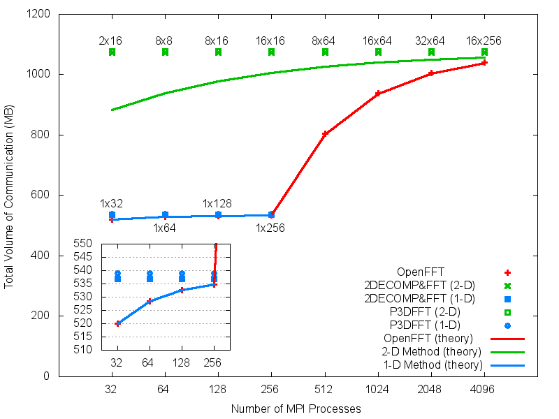
(a) Theoretical and practical volumes of communication (256^3). The practical volume is reported by the MPI profiler on the K computer.
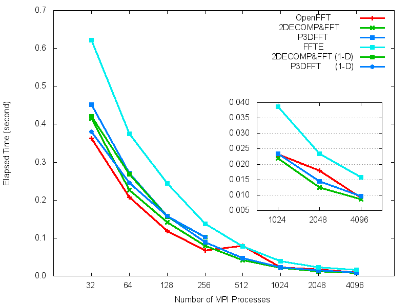
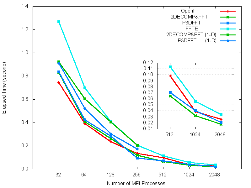
(b) Cray XC30 (512^3).
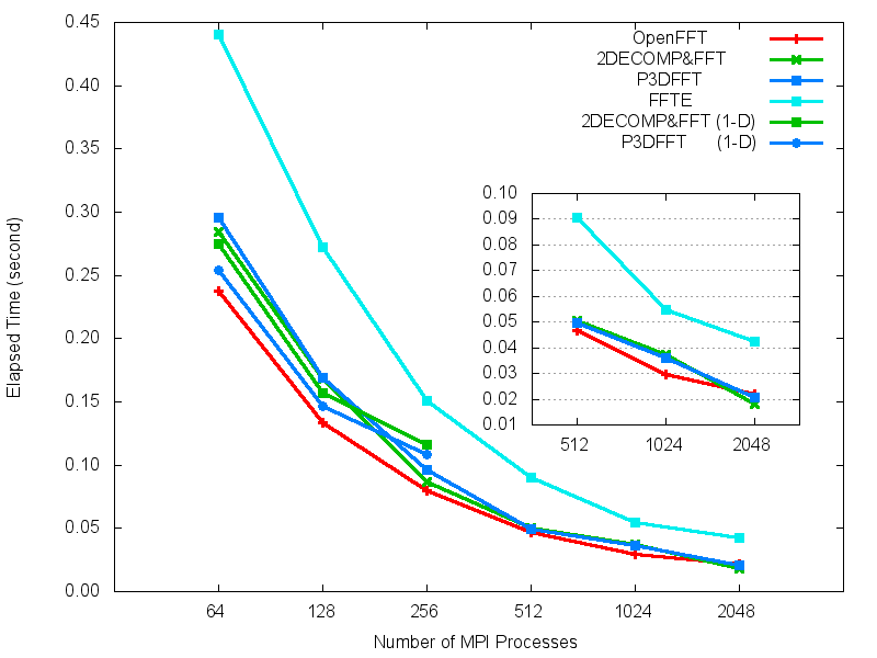
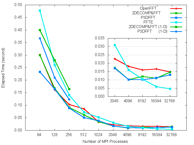
(c) SGI InfiniBand Machine (512^3).
(d) Fujitsu FX10 (512^3).
(e) K computer (512^3).