Macroscopic polarization by Berry's phase

The macroscopic electric polarization of a bulk system can be calculated based on the Berry phase formalism [15]. As an example, let us illustrate a calculation of a Born effective charge of Na in a NaCl bulk via the macroscopic polarization.
(1) SCF calculation
First, perform a conventional SCF calculation using an input file 'NaCl.dat' in the directory 'work'. Then, the following keyword 'HS.fileout' should be switched on

    HS.fileout               on     # on|off, default=off

When the calculation is completed normally, then you can find an output file 'nacl.scfout' in the directory 'work'.

(2) Calculation of macroscopic polarization
The macroscopic polarization is calculated by a post-processing code 'polB' of which input data is 'nacl.scfout'. In the directory 'source', please compile as follows:

    % make polB

When the compilation is completed normally, then you can find an executable file 'polB' in the directory 'work'. Then, please move to the directory 'work', and perform as follows:

    % polB nacl.scfout
   or
    % polB nacl.scfout < in > out

In the latter case, the file 'in' contains the following ingredients:

    9 9 9
    1 1 1

In the former case, you will be interactively asked from the program as follows:

******************************************************************
******************************************************************
 polB:
 code for calculating the electric polarization of bulk systems
 Copyright (C), 2006-2007, Fumiyuki Ishii and Taisuke Ozaki 
 This is free software, and you are welcome to         
 redistribute it under the constitution of the GNU-GPL.
******************************************************************
******************************************************************

Read the scfout file (nacl.scfout)
 Previous eigenvalue solver = Band
 atomnum                    = 2
 ChemP                      = -0.156250000000 (Hartree)
 E_Temp                     = 300.000000000000 (K)
 Total_SpinS                =  0.000000000000 (K)
 Spin treatment             = collinear spin-unpolarized

 r-space primitive vector (Bohr)
  tv1=  0.000000   5.319579   5.319579
  tv2=  5.319579   0.000000   5.319579
  tv3=  5.319579   5.319579   0.000000
 k-space primitive vector (Bohr^-1)
  rtv1= -0.590572   0.590572   0.590572
  rtv2=  0.590572  -0.590572   0.590572
  rtv3=  0.590572   0.590572  -0.590572

  Cell_Volume=301.065992 (Bohr^3)

 Specify the number of grids to discretize reciprocal a-, b-, and c-vectors
 (e.g 2 4 3)
   k1    0.00000    0.11111    0.22222    0.33333    0.44444  ...
   k2    0.00000    0.11111    0.22222    0.33333    0.44444  ...
   k3    0.00000    0.11111    0.22222    0.33333    0.44444  ...

 Specify the direction of polarization as reciprocal a-, b-, and c-vectors
 (e.g 0 0 1 ) 1 1 1

Then, the calculation will start like this:

calculating the polarization along the a-axis ....
The number of strings for Berry phase : AB mesh=81

  calculating the polarization along the a-axis ....   1/  82
  calculating the polarization along the a-axis ....   2/  82 
  .....
  ...

*******************************************************
              Electric dipole  (Debye) : Berry phase
*******************************************************

 Absolute dipole moment      163.93373639

               Background        Core             Electron          Total

 Dx           -0.00000000       94.64718996       -0.00000338       94.64718658
 Dy           -0.00000000       94.64718996       -0.00000283       94.64718713
 Dz           -0.00000000       94.64718996       -0.00000317       94.64718679


***************************************************************
              Electric polarization (muC/cm^2) : Berry phase
***************************************************************

               Background        Core             Electron          Total

 Px           -0.00000000      707.66166752       -0.00002529      707.66164223
 Py           -0.00000000      707.66166752       -0.00002118      707.66164633
 Pz           -0.00000000      707.66166752       -0.00002371      707.66164381


Elapsed time = 77.772559 (s) for myid=  0

Since the Born effective charge $Z_{\alpha\beta}^{*}$ is defined by a tensor:

$\displaystyle Z_{\alpha\beta}^{*} = \frac{V_{c}}{\vert e \vert}\frac{\Delta P_{\alpha}}{\Delta u_{\beta}}$

where $V_{c}$ is the volume of the unit cell,

the elementary charge, $\Delta u_{\beta}$ displacement along $\beta$ -coordinate, $\Delta P_{\alpha}$ the change of macroscopic polarization along $\alpha$ -coordinate, therefore we will perform the above procedures (1) and (2) at least two or three times by varying the

, or

-coordinate of Na atom. Then, for example, we have along

-coordinates

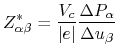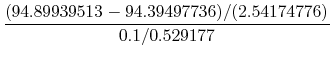
    Px = 94.39497736 (Debye/unit cell) at x= -0.05 (Ang)
    Px = 94.64718658 (Debye/unit cell) at x=  0.0  (Ang)
    Px = 94.89939513 (Debye/unit cell) at x=  0.05 (Ang)

Thus,

$\displaystyle Z^{*}_{xx}$	$\textstyle =$	$\displaystyle \frac{(94.89939513-94.39497736)/(2.54174776)}{0.1/0.529177}$
	$\textstyle =$	$\displaystyle 1.050$

**Table 7:** Calculated Born effective charge of Na in a NaCl bulk. The input file is 'NaCl.dat' in the directory 'work'. Another theoretical value (FD: Ref. [116]) and experimental value (Ref. [117]) are also shown for comparison.
	OpenMX	FD	Expt.
	1.05	1.09	1.12

Note that in the NaCl bulk the off-diagonal terms in the tensor of Born charge are zero, and $Z^{*}_{xx}=Z^{*}_{yy}=Z^{*}_{zz}$ . In Table 7 we see that the calculated value is in good agreement with the other calculation [116] and an experimental result [117]. The calculation of macroscopic polarization is supported for both the collinear and non-collinear DFT. It is also noted that the code 'polB' has been parallelized for large-scale systems where the number of processors can exceed the number of atoms in the system.