Next: Analysis of difference in Up: User's manual of OpenMX Previous: Delta factor Contents Index
The Fermi surface is visualized by XCrySDen [66]. When you perform calculations of the density of states by the following keywords:
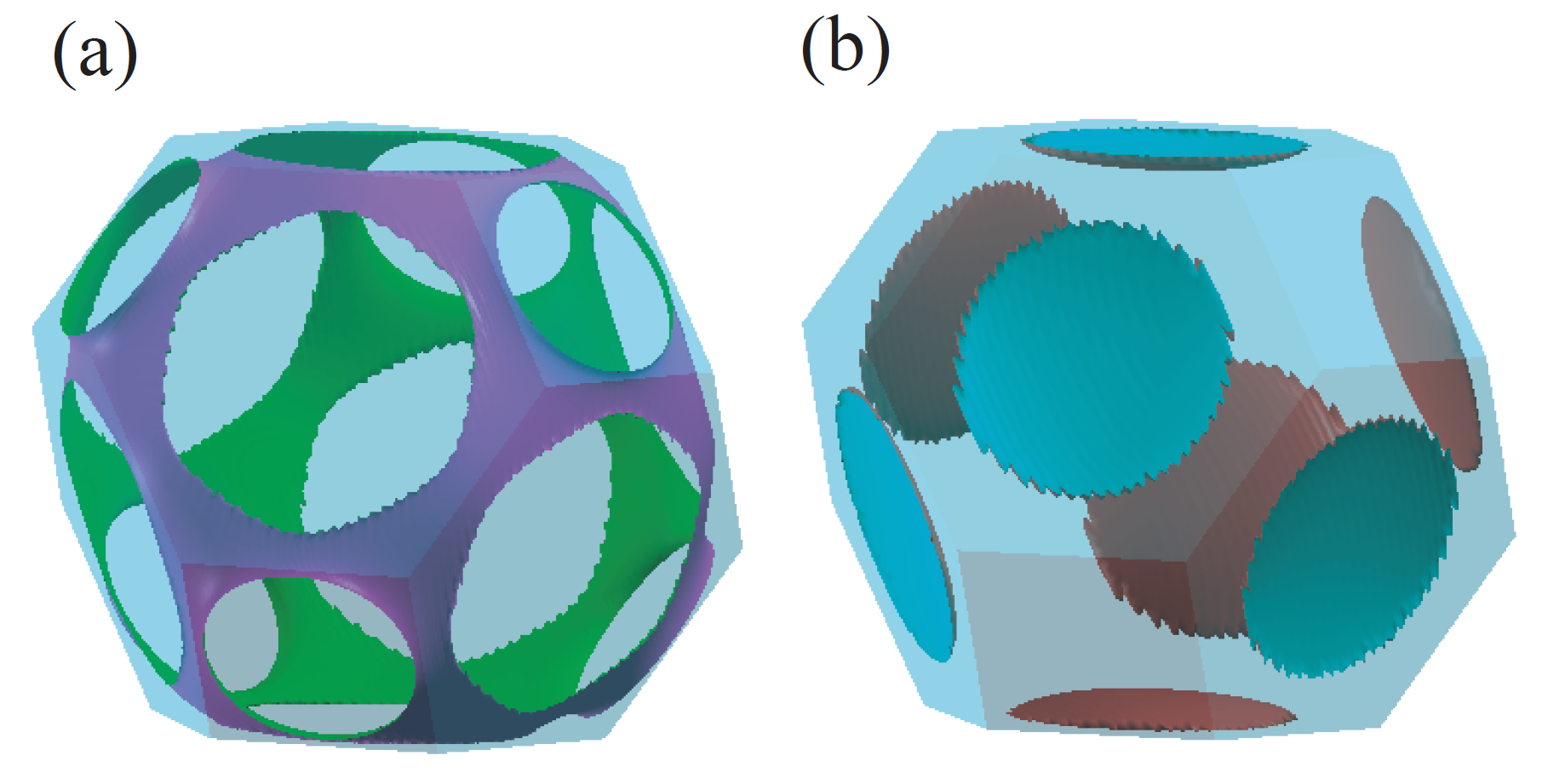
  Dos.fileout                  on        # on|off, default=off
  Dos.Erange              -20.0  20.0    # default = -20 20
  Dos.Kgrid                 61 61 61     # default = Kgrid1 Kgrid2 Kgrid3
you will obtain a file 'System.Name.FermiSurf0.bxsf', where 'System.Name' is 'System.Name', and the file can be visualized by XCrySDen [66]. As well as 'Dos.Fileout', 'DosGauss.fileout' can be also used for the purpose. In case of spin-polarized calculations, two files are generated as 'System.Name.FermiSurf0.bxs' and 'System.Name.FermiSurf1.bxs' for spin-up and spin-down states, respectively. In case of non-collinear calculations, a file 'System.Name.FermiSurf.bxs' is generated. It is noted that a large number of k-points should be used in order to obtain a smooth Fermi surface. As an example, Fermi surfaces of the fcc Ca bulk are shown in Fig. 54. The input file used for the calculation is 'Cafcc_FS.dat' in the directory 'work'.
 |
2016-04-03