Next: Restarting the NEB calculation Up: Nudged elastic band (NEB) Previous: How to perform Contents Index
Two input files are provided as example:
Cycloaddition reaction of two ethylene molecules to cyclobutane
Diffusion of an interstitial hydrogen atom in the diamond Si
The input file 'C2H4_NEB.dat' will be used to illustrate the NEB calculation in the proceeding explanation.
Providing two terminal structures
The atomic coordinates of the precursor are specified in the input file by
  <Atoms.SpeciesAndCoordinates
  1    C   -0.66829065594143    0.00000000101783   -2.19961193219289     2.0     2.0
  2    C    0.66817412917689   -0.00000000316062   -2.19961215251205     2.0     2.0
  3    H    1.24159214112072   -0.92942544650857   -2.19953308980064     0.5     0.5
  4    H    1.24159212192367    0.92942544733979   -2.19953308820323     0.5     0.5
  5    H   -1.24165800644131   -0.92944748269232   -2.19953309891389     0.5     0.5
  6    H   -1.24165801380425    0.92944749402510   -2.19953309747076     0.5     0.5
  7    C   -0.66829065113509    0.00000000341499    2.19961191775648     2.0     2.0
  8    C    0.66817411530651   -0.00000000006073    2.19961215383949     2.0     2.0
  9    H    1.24159211310925   -0.92942539308841    2.19953308889301     0.5     0.5
  10    H    1.24159212332935    0.92942539212392    2.19953308816332     0.5     0.5
  11    H   -1.24165799549343   -0.92944744948986    2.19953310195071     0.5     0.5
  12    H   -1.24165801426648    0.92944744880542    2.19953310162389     0.5     0.5
  Atoms.SpeciesAndCoordinates>
  <NEB.Atoms.SpeciesAndCoordinates
  1    C   -0.77755846408657   -0.00000003553856   -0.77730141035137     2.0     2.0
  2    C    0.77681707294741   -0.00000002413166   -0.77729608216595     2.0     2.0
  3    H    1.23451821718817   -0.88763832172374   -1.23464057728123     0.5     0.5
  4    H    1.23451823170776    0.88763828275851   -1.23464059022330     0.5     0.5
  5    H   -1.23506432458023   -0.88767426830774   -1.23470899088096     0.5     0.5
  6    H   -1.23506425800395    0.88767424658723   -1.23470896874564     0.5     0.5
  7    C   -0.77755854665393    0.00000000908006    0.77730136931056     2.0     2.0
  8    C    0.77681705017323   -0.00000000970885    0.77729611199476     2.0     2.0
  9    H    1.23451826851556   -0.88763828740000    1.23464060936812     0.5     0.5
  10    H    1.23451821324627    0.88763830875131    1.23464061208483     0.5     0.5
  11    H   -1.23506431230451   -0.88767430754577    1.23470894717613     0.5     0.5
  12    H   -1.23506433587007    0.88767428525317    1.23470902573029     0.5     0.5
  NEB.Atoms.SpeciesAndCoordinates>
Keywords for the NEB calculation
The NEB calculation can be performed by setting the keyword 'MD.Type' as
MD.Type NEB
The number of images in the path is given by
MD.NEB.Number.Images 8 # default=10
The spring constant is given by
MD.NEB.Spring.Const 0.1 # default=0.1(hartee/borh^2)
The optimization of MEP is performed by a hybrid DIIS+BFGS scheme which is controlled by the following keywords:
  MD.Opt.DIIS.History           4          # default=7
  MD.Opt.StartDIIS             10          # default=5
  MD.maxIter                  100          # default=1
  MD.Opt.criterion         1.0e-4          # default=1.0e-4 (Hartree/Bohr)
Execution of the NEB calculation
One can perform the NEB calculation with the input file 'C2H4_NEB.dat' by
% mpirun np 16 openmx C2H4_NEB.datIf the calculation is successfully completed, more than 24 files will be generated. Some of them are listed below:
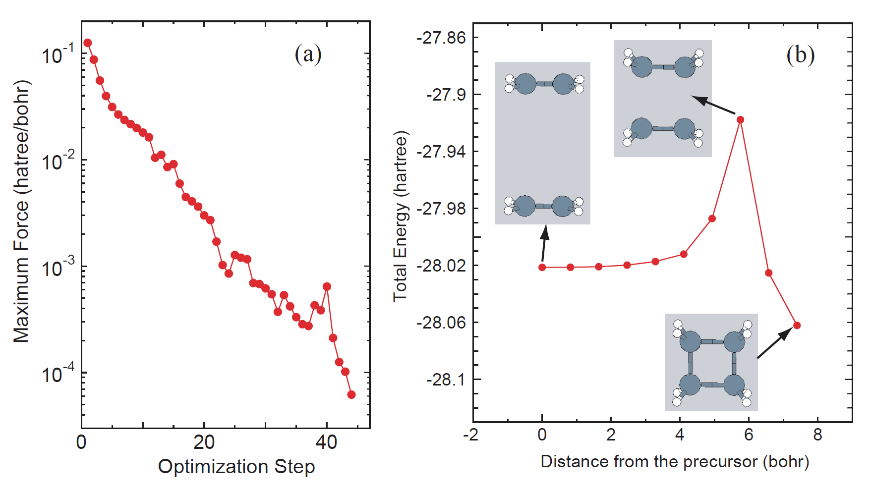
  c2h4.neb.opt          history of optimization for finding MEP
  c2h4.neb.ene          total energy of each image
  c2h4.neb.xyz          atomic coordinates of each image in XYZ format
  C2H4_NEB.dat#         input file for restarting.
  C2H4_NBE.dat_0        input file for the precursor
  C2H4_NBE.dat_1        input file for the image 1
  C2H4_NBE.dat_2        input file for the image 2
  C2H4_NBE.dat_3        input file for the image 3
  C2H4_NBE.dat_4        input file for the image 4
  C2H4_NBE.dat_5        input file for the image 5
  C2H4_NBE.dat_6        input file for the image 6
  C2H4_NBE.dat_7        input file for the image 7
  C2H4_NBE.dat_8        input file for the image 8
  C2H4_NBE.dat_9        input file for the product
  c2h4_0.out            output file for the precursor
  c2h4_1.out            output file for the image 1
  c2h4_2.out            output file for the image 2
  c2h4_3.out            output file for the image 3
  c2h4_4.out            output file for the image 4
  c2h4_5.out            output file for the image 5
  c2h4_6.out            output file for the image 6
  c2h4_7.out            output file for the image 7
  c2h4_8.out            output file for the image 8
  c2h4_9.out            output file for the product
'c2h4.neb.opt' contains history of optimization for finding MEP as shown in Fig. 45(a). One can see the details at the header of the file as follows:
  ***********************************************************
  ***********************************************************
  History of optimization by the NEB method
  ***********************************************************
  ***********************************************************

  iter   SD_scaling     |Maximum force|   Maximum step        Norm        Sum of Total Energy of Images
  (Hartree/Bohr)        (Ang)       (Hartree/Bohr)       (Hartree)

  1       0.37794520       0.12552253       0.04583483       0.49511548    -223.77375997
  2       0.37794520       0.08735938       0.03172307       0.35373414    -223.85373393
  3       0.37794520       0.05559291       0.01919790       0.25650527    -223.89469352
  4       0.37794520       0.03970051       0.01254863       0.20236344    -223.91689564
  5       0.45353424       0.03132536       0.01360864       0.17275416    -223.93128189
  6       0.45353424       0.02661456       0.01202789       0.15142709    -223.94412534
  7       0.45353424       0.02367627       0.01068250       0.13703973    -223.95422398
  .....
  ...
  .
Also, 'c2h4.neb.ene' and 'c2h4.neb.xyz' can be used to analyze the change of total energy as a function of the distance (Bohr) from the precursor and the structural change as shown in Fig. 46(b). The content of 'c2h4.neb.ene' is as follows:
  #
  # 1st column: index of images, where 0 and MD.NEB.Number.Images+1 are the terminals
  # 2nd column: Total energy (Hartree) of each image
  # 3rd column: distance (Bohr) between neighbors
  # 4th column: distance (Bohr) from the image of the index 0
  #
  0     -28.02131967       0.00000000       0.00000000
  1     -28.02125585       0.82026029       0.82026029
  2     -28.02086757       0.82124457       1.64150486
  3     -28.01974890       0.82247307       2.46397794
  4     -28.01724274       0.82231749       3.28629543
  5     -28.01205847       0.82220545       4.10850088
  6     -27.98707448       0.82271212       4.93121300
  7     -27.91765377       0.82175187       5.75296486
  8     -28.02520689       0.82164937       6.57461423
  9     -28.06207901       0.82095145       7.39556568
where the first column is a serial number of image, while 0 and 9 correspond to the precursor and product, respectively. The second column is the total energy of each image. The third and fourth columns are interval (Bohr) between two neighboring images and the distance (Bohr) from the precursor in geometrical phase space.
 |
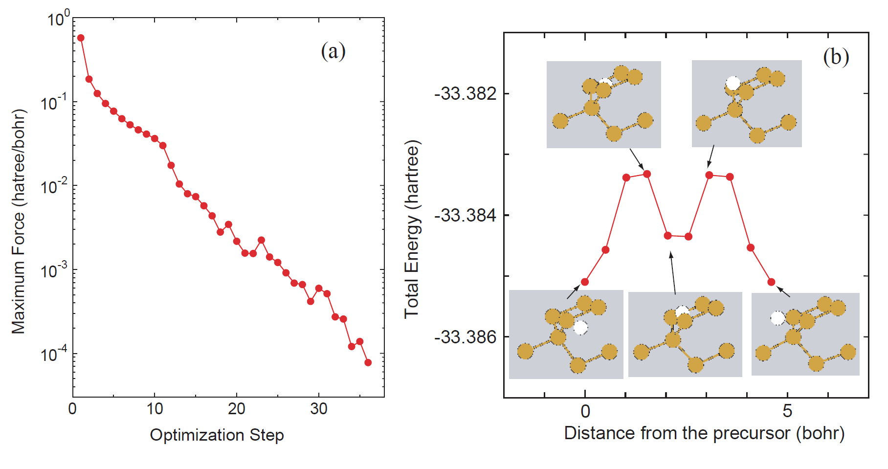
As well as the case of 'C2H4_NEB.dat', one can perform the NEB calculation by 'Si8_NEB.dat'. After the successful calculation, you may get the history of optimization and change of total energy along MEP as shown in Fig. 47.
 |