Next: 交換結合パラメータ Up: OpenMX Ver. 3.7 ユーザーマニュアル Previous: 軌道磁気モーメントに対するZeeman項 Contents Index

Berry位相による巨視的分極の計算

Berry位相の方法を用いて、バルクの巨視的電気分極を計算することができます [12]。例として、塩化ナトリウム中のナトリウム原子のBorn有効電荷を巨視的電気分極から計算する手順を説明します。

(1) SCF計算

最初に、「work」ディレクトリ中にある入力ファイル「NaCl.dat」を用いて、通常のSCF計算を実行します。この際に、キーワード「HS.fileout」をオンにします。

    HS.fileout               on     # on|off, default=off

SCF計算が正常に完了すると、「work」ディレクトリ中に出力ファイル「nacl.scfout」が生成されます。

(2) 巨視的分極の計算

巨視的分極はポストプロセスのプログラム「polB」を用いて計算します。この際に「nacl.scfout」が入力データとなります。まず「source」ディレクトリにおいて、「polB」を次のようにコンパイルします。

    % make polB

コンパイルが正常に完了すると、「work」ディレクトリ中に実行形式ファイル「polB」が生成されます。次に、「work」ディレクトリに移動し、次のように実行します。

    % polB nacl.scfout
   もしくは
    % polB nacl.scfout < in > out

後者の場合、テキストファイル「in」には次のデータが保存されています。

    9 9 9
    1 1 1

前者の場合、次のように会話形式でプログラムから質問されます。

******************************************************************
******************************************************************
 polB:
 code for calculating the electric polarization of bulk systems
 Copyright (C), 2006-2007, Fumiyuki Ishii and Taisuke Ozaki 
 This is free software, and you are welcome to         
 redistribute it under the constitution of the GNU-GPL.
******************************************************************
******************************************************************

Read the scfout file (nacl.scfout)
 Previous eigenvalue solver = Band
 atomnum                    = 2
 ChemP                      = -0.156250000000 (Hartree)
 E_Temp                     = 300.000000000000 (K)
 Total_SpinS                =  0.000000000000 (K)
 Spin treatment             = collinear spin-unpolarized

 r-space primitive vector (Bohr)
  tv1=  0.000000   5.319579   5.319579
  tv2=  5.319579   0.000000   5.319579
  tv3=  5.319579   5.319579   0.000000
 k-space primitive vector (Bohr^-1)
  rtv1= -0.590572   0.590572   0.590572
  rtv2=  0.590572  -0.590572   0.590572
  rtv3=  0.590572   0.590572  -0.590572

  Cell_Volume=301.065992 (Bohr^3)

 Specify the number of grids to discretize reciprocal a-, b-, and c-vectors
 (e.g 2 4 3) 9 9 9
   k1    0.00000    0.11111    0.22222    0.33333    0.44444  ...
   k2    0.00000    0.11111    0.22222    0.33333    0.44444  ...
   k3    0.00000    0.11111    0.22222    0.33333    0.44444  ...

 Specify the direction of polarization as reciprocal a-, b-, and c-vectors
 (e.g 0 0 1 ) 1 1 1

逆格子ベクトルの離散化グリッド数と分極の方向を指定した後に、計算が以下のように進行します。

calculating the polarization along the a-axis ....
The number of strings for Berry phase : AB mesh=81

  calculating the polarization along the a-axis ....   1/  82
  calculating the polarization along the a-axis ....   2/  82 
  .....
  ...

*******************************************************
              Electric dipole  (Debye) : Berry phase
*******************************************************

 Absolute dipole moment      163.93373639

               Background        Core             Electron          Total

 Dx           -0.00000000       94.64718996       -0.00000338       94.64718658
 Dy           -0.00000000       94.64718996       -0.00000283       94.64718713
 Dz           -0.00000000       94.64718996       -0.00000317       94.64718679


***************************************************************
              Electric polarization (muC/cm^2) : Berry phase
***************************************************************

               Background        Core             Electron          Total

 Px           -0.00000000      707.66166752       -0.00002529      707.66164223
 Py           -0.00000000      707.66166752       -0.00002118      707.66164633
 Pz           -0.00000000      707.66166752       -0.00002371      707.66164381


Elapsed time = 77.772559 (s) for myid=  0

$V_{c}$ を単位セルの体積、

を素電荷、 $\Delta u_{\beta}$ を $\beta$ 座標方向の変位、 $\Delta P_{\alpha}$ を $\alpha$ 座標方向の巨視的分極の変化とすると、 Born有効電荷 $Z_{\alpha\beta}^{*}$ は次のようにテンソルで定義されます。

$\displaystyle Z_{\alpha\beta}^{*} = \frac{V_{c}}{\vert e \vert}\frac{\Delta P_{\alpha}}{\Delta u_{\beta}}$

上記の表式に従い、Born有効電荷を計算する際には、ナトリウム原子の

、

座標を変化させながら、上の手順を少なくとも2回もしくは3回実行します。例えば

座標方向を変位させて分極を計算すると、次の結果が得られます。

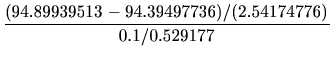
    Px = 94.39497736 (Debye/unit cell) at x= -0.05 (Ang)
    Px = 94.64718658 (Debye/unit cell) at x=  0.0  (Ang)
    Px = 94.89939513 (Debye/unit cell) at x=  0.05 (Ang)

したがって、ナトリウム原子のBorn有効電荷は以下のように計算されます。

$\displaystyle Z^{*}_{xx}$	$\textstyle =$	$\displaystyle \frac{(94.89939513-94.39497736)/(2.54174776)}{0.1/0.529177}$
	$\textstyle =$	$\displaystyle 1.050$

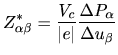
塩化ナトリウム固体では、Born電荷のテンソルの非対角項はゼロ、そして $Z^{*}_{xx}=Z^{*}_{yy}=Z^{*}_{zz}$ となります。表5に、ここでの計算値と他の計算値 [72]および実験値[73]との比較を示します。計算値と実験値が良く一致していることが分かります。巨視的分極の計算はコリニアおよびノンコリニアDFT法の両者に対してサポートされています。またMPIプロセス数が系の原子数を上回る場合でも、プログラム「polB」は効率的な並列計算が可能です。

**Table 5:** Berry位相による巨視的分極の計算から見積もられたNaCl中のNaのBorn有効電荷。入力ファイルは「work」ディレクトリ中の「NaCl.dat」。比較のため、他の計算値(FD: 参考文献[72])と実験値(参考文献[73])も併記。
	OpenMX	FD	Expt.
	1.05	1.09	1.12

t-ozaki 2013-12-23