Orbital optimization

The radial function of basis orbitals can be variationally optimized using the orbital optimization method [26]. As an illustration of the orbital optimization, let us explain it using a methane molecule of which input file is Methane_OO.dat. In the orbital optimization method the optimized orbitals are expressed by the linear combination of primitive orbitals, and obtained by variationally optimizing the contraction coefficients. The number of the primitive and optimized orbitals in the optimization are specified by

    <Definition.of.Atomic.Species
      H   H5.0-s4>1            H_CA11
      C   C5.0-s4>1p4>1        C_CA11
    Definition.of.Atomic.Species>

For 'H' one optimized radial function for the s-orbital is obtained from the linear combination of four primitive radial functions. Similary, one optimized radial function for the s-(p-)orbital is obtained from the linear combination of four primitive radial functions for 'C'. In addition, the following keywords are set in the input file as follows:

    orbitalOpt.Method          species     # Off|Species|Atoms
    orbitalOpt.Opt.Method        EF        # DIIS|EF
    orbitalOpt.SD.step        0.001        # default=0.001
    orbitalOpt.HistoryPulay     30         # default=15
    orbitalOpt.StartPulay       10         # default=1
    orbitalOpt.scf.maxIter      60         # default=40
    orbitalOpt.Opt.maxIter     140         # default=100
    orbitalOpt.per.MDIter       20         # default=1000000
    orbitalOpt.criterion      1.0e-4       # default=1.0e-4 

    CntOrb.fileout               on        # on|off, default=off
    Num.CntOrb.Atoms             2         # default=1
    <Atoms.Cont.Orbitals
     1
     2
    Atoms.Cont.Orbitals>

Then, we execute OpenMX as:

    % ./openmx Methane_OO.dat
  

When the execution is completed normally, you can find the history of orbital optimization in the file 'met_oo.out' as:

***********************************************************
***********************************************************
         History of orbital optimization   MD= 1
*********     Gradient Norm ((Hartree/borh)^2)     ********
              Required criterion=  0.000100000000
***********************************************************

   iter=   1  Gradient Norm=  0.057099116186  Uele= -3.217165688850
   iter=   2  Gradient Norm=  0.044668590658  Uele= -3.220124728727
   iter=   3  Gradient Norm=  0.034308424834  Uele= -3.223127810870
   iter=   4  Gradient Norm=  0.025847684906  Uele= -3.226182452559
   iter=   5  Gradient Norm=  0.019106482737  Uele= -3.229299561866
   iter=   6  Gradient Norm=  0.013893901444  Uele= -3.232493788494
   iter=   7  Gradient Norm=  0.010499563363  Uele= -3.235308811420
   iter=   8  Gradient Norm=  0.008362684115  Uele= -3.237657609355
   iter=   9  Gradient Norm=  0.006959746319  Uele= -3.239623291338
   iter=  10  Gradient Norm=  0.005994856595  Uele= -3.241273216875
   iter=  11  Gradient Norm=  0.005298132389  Uele= -3.242661771498
   iter=  12  Gradient Norm=  0.003059669828  Uele= -3.250897736701
   iter=  13  Gradient Norm=  0.001390212138  Uele= -3.255127796347
   iter=  14  Gradient Norm=  0.000781057925  Uele= -3.255185826155
   iter=  15  Gradient Norm=  0.000726780237  Uele= -3.255269791193
   iter=  16  Gradient Norm=  0.000390997436  Uele= -3.250876275966
   iter=  17  Gradient Norm=  0.000280772241  Uele= -3.250340948913
   iter=  18  Gradient Norm=  0.000200449371  Uele= -3.252358609122
   iter=  19  Gradient Norm=  0.000240967733  Uele= -3.254237590017
   iter=  20  Gradient Norm=  0.000081978704  Uele= -3.258145769943

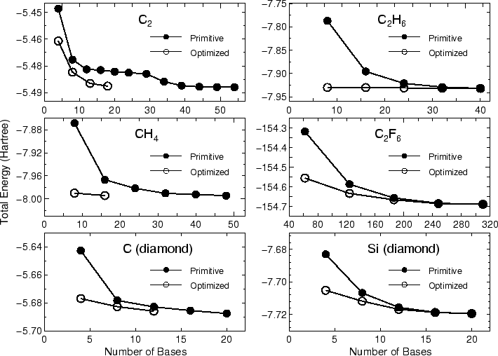
In most cases, 20-50 iterative steps are enough to achieve a sufficient convergence. The comparison between the primitive basis orbitals and the optimized orbitals in the total energy is given by

    Primitive basis orbitals
       Utot  =      -7.992568903114 (Hartree) 

    Optimized orbitals by the orbital optimization 
       Utot  =      -8.133746206187 (Hartree)

Figure 14: The total energy for a carbon dimer C$_2$, a methane molecule CH$_4$, carbon and silicon in the diamond structure, a ethane molecule C$_2$H$_6$, and a hexafluoro ethane molecule C$_2$F$_6$ as a function of the number of primitive and optimized orbitals. The total energy and the number of orbitals are defined as those per atom for C$_2$, carbon and silicon in the diamond, and as those per molecule for CH$_4$, C$_2$H$_6$, and C$_2$F$_6$.

We see that the small but accurate basis set orbitals can be generated by the orbital optimization. In Fig. 14 we show the convergence properties of total energies for molecules and bulks as a function of the number of unoptimized and optimized orbitals. We see that a remarkable convergent results are obtained using the optimized orbitals for all systems. In this illustration of a methane molecule, the optimized radial orbitals are output to files, C_1.pao and H_2.pao. These output files, C_1.pao and H_2.pao, could be an input data for pseudo-atomic orbitals as it is. This means that it is possible to perform a pre-optimization of basis orbitals for systems you are interested in. The pre-optimization could be performed for smaller but chemically similar systems.

The following two options are available for the keyword 'orbitalOpt.Method', 'atoms' in which basis obitals on each atom are fully optimized, 'species' in which basis obitals on each species are optimized.

• atoms

  The radial functions of basis orbitals are optimized with a constraint that the radial wave function $R$ is independent on the magnetic quantum number, which guarantees the rotational invariance of the total energy. However, the optimized orbital on all the atoms can be different eath other.

• species

  Basis orbitals in atoms with the same species name, that you define in 'Definition.of.Atomic.Species', are optimized as the same orbitals. If you want to assign the same orbitals to atoms with almost the same chemical environment, and optimize these orbitals, this scheme could be quite convenient.

Although the same information is available in the section 'Input file', for convenience the details of the other keywords are listed below:
orbitalOpt.scf.maxIter
The maximum number of SCF iterations in the orbital optimization is specified by the keyword 'orbitalOpt.scf.maxIter'.

orbitalOpt.Opt.maxIter
The maximum number of iterations for the orbital optimization is specified by the keyword 'orbitalOpt.Opt.maxIter'. The iteration loop for the orbital optimization is terminated at the number specified by 'orbitalOpt.Opt.maxIter' even when a convergence criterion is not satisfied.

orbitalOpt.Opt.Method
Two schemes for the optimization of orbitals are available: 'EF' which is an eigenvector following method, 'DIIS' which is the direct inversion method in iterative subspace. The algorithms are basically same as for the geometry optimization. Either 'EF' or 'DIIS' is chosen by the keyword, 'orbitalOpt.Opt.Method'.

orbitalOpt.StartPulay
The quasi Newton method, 'EF' and 'DIIS' starts from the optimization step specified by the keyword 'orbitalOpt.StartPulay'.

orbitalOpt.HistoryPulay
The keyword 'orbitalOpt.HistoryPulay' specifies the number of previous steps to estimate the next input contraction coefficients used in the quasi Newton method, 'EF' and 'DIIS'.

orbitalOpt.SD.step
Steps before moving the quasi Newton method, 'EF' and 'DIIS' is performed by the steepest decent method. The prefactor used in the steepest decent method is specified by the keyword 'orbitalOpt.SD.step'. In most cases, orbitalOpt.SD.step of 0.001 can be a good prefactor.

orbitalOpt.criterion
The keyword 'orbitalOpt.criterion' specifies a convergence criterion ((Hartree/borh)$^2$) for the orbital optimization. The iterations loop is finished when a condition, Norm of derivatives$<$orbitalOpt.criterion, is satisfied.

CntOrb.fileout
If you want to output the optimized radial orbitals to files, then the keyword 'CntOrb.fileout' must be ON.

Num.CntOrb.Atoms
The keyword 'Num.CntOrb.Atoms' gives the number of atoms whose optimized radial orbitals are output to files.

Atoms.Cont.Orbitals
The keyword 'Atoms.Cont.Orbitals' specifies the atom number, which was given by the first column in the specification of the keyword 'Atoms.SpeciesAndCoordinates' for the output of optimized orbitals as follows:

    <Atoms.Cont.Orbitals
     1
     2
    Atoms.Cont.Orbitals>

The beginning of the description must be '$<$Atoms.Cont.Orbitals', and the last of the description must be 'Atoms.Cont.Orbitals$>$'. The number of lines should be consistent with the number specified in the keyword 'Atoms.Cont.Orbitals'. For example, the name of files are C_1.pao and H_2.pao, where the symbol corresponds to that given by the first column in the specification of the keyword 'Definition.of.Atomic.Species' and the number after the symbol means that of the first column in the specification of the keyword 'Atoms.SpeciesAndCoordinates'. These outout files, C_1.pao and H_2.pao, can be an input data for pseudo-atomic orbitals as it is.